Introduction
Functional magnetic resonance imaging (fMRI) has established itself as a key tool in the field of auditory neuroscience. However, designing auditory fMRI experiments poses unique challenges due to the substantial noise generated by the rapid switching of gradient coils during echo planar imaging (EPI), which can reach up to 120 dB SPL. In a typical continuous EPI sequence, scans are continuously collected while stimuli are presented alongside the noise generated by the scanner, which offers the advantage of maximizing data collection and preserving fMRI temporal resolution. However, the scanner noise interferes with the stimulus and partially saturates the response of the auditory cortex, limiting the dynamic range available for detecting stimulus-related brain activity (Edmister et al., 1999). Moreover, in the context of speech-related tasks, the decreased acoustic clarity caused by the scanner noise increases cognitive load, significantly impacting fMRI sensitivity and data interpretation (Peelle, 2014).
The typical approach to protecting human participants from scanner noise is to use passive sound attenuation, e.g. using over-ear hearing protection in conjunction with foam earplugs, insert earphones, and/ or active noise control. This results in a maximum total noise reduction of approximately 40 dB (Hall et al., 2009; Ravicz & Melcher, 2001). Despite such protective measures, a substantial amount of noise is still transmitted to the cochlea, either through the tympani or by bone conduction. Consequently, the stimulus is perceived differently when presented along with the scanner noise or in quiet conditions. This may be acceptable depending on the stimuli and the brain regions being examined. However, presenting stimuli in silence can be crucial when frequency ranges of the stimuli and EPI noise significantly overlap (Langers et al., 2014); when small alterations in the stimuli spectra result in large perceptual changes (Trapeau & Schönwiesner, 2018); when comparisons across experimental conditions require fine-grained acoustic discrimination; or, more critically, when the experimental setup does not allow for optimal acoustic protection of the subjects, as is often the case in animal research.
The classical method to presenting auditory stimuli that are not masked by the scanner noise, sparse sampling, involves separating volume acquisitions by a long gap (10 to 16 s) that allows for the presentation of sound stimuli in silence, and exploits the fact that the peak of the hemodynamic response occurs several seconds after the stimulus (Belin et al., 1999; Hall et al., 1999). Furthermore, the long silent intervals avoid contamination by the hemodynamic response to the scanner noise and allow for complete recovery of the magnetization from one volume acquisition to the next. Sparse sampling has been extensively used when studying primary auditory cortex (A1) and subcortical areas (Fuglsang et al., 2022; Oya et al., 2018; Trapeau & Schönwiesner, 2015; Wolak et al., 2017), as well as higher-level areas in both humans and animal studies (Bach et al., 2013; Belin & Zatorre, 2003; Joly et al., 2012; Ortiz-Rios et al., 2015; Petkov et al., 2008; Schönwiesner et al., 2015). Comparisons of sparse and continuous sequences comprising the same number of volumes emphasized the detrimental effect of scanner background noise. Identical sound stimulation sequences evoked higher signal in primary and higher-order auditory regions (Gaab et al., 2007), as well as in other intrinsic networks (Yakunina et al., 2015), when data were acquired with sparse sampling compared to a subset of the scan data acquired during continuous scanning that exactly matched the data sampling during sparse acquisition. Sparse sampling also elicits greater response in rhesus macaque auditory areas compared to a continuous sequence with the same number of volumes but a shorter duration (Petkov et al., 2009). In contrast, duration-matched comparisons of both protocols yielded divergent results. Continuous paradigms exhibited a significantly larger extent of activation when compared to duration-matched versions of the sparse paradigm (Dewey et al., 2021; Hall et al., 2014; Peelle et al., 2010). These results can be attributed to the primary limitation of sparse sampling, namely the relatively low number of images acquired per time unit. Furthermore, sparse sampling only provides a single measure per stimulus, which precludes the assessment of the profile of the hemodynamic response without scanning each stimulus multiple times with jittered intervals.
Clustered sparse sampling is a hybrid method that combines the advantages of sparse sampling with more efficient data acquisition. In this protocol, multiple fMRI volumes are acquired in rapid succession (a "cluster") after a silent period, allowing for greater temporal coverage and statistical power than classical sparse sampling while still preserving relatively long moments of silence for stimulus presentation. Duration-matched comparisons between sparse and clustered sparse protocols, using clusters of three volumes, showed significantly enhanced functional responses along the superior temporal plane (Schmidt et al., 2008; Zaehle et al., 2007) for the clustered sparse protocol. However, a drawback of this method is that longitudinal magnetization does not reach a steady state within the acquisition of a single cluster, resulting in a T1 signal decay over the course of the cluster acquisition. To address the issue of T1-decay, various corrective approaches have been employed. These include the incorporation of regressors to model the decay (Schmidt et al., 2008; Zaehle et al., 2007), the averaging of the volumes within each cluster (Riecke et al., 2017; Riecke et al., 2018), and the analysis of each volume within a cluster as a distinct session (Keil et al., 2020; Stewart et al., 2022; Zaehle et al., 2004)
To entirely prevent T1-decay during clustered sparse data acquisition, longitudinal magnetization can be maintained in a steady state during pseudo-quiet periods, by maintaining silent slice-selective excitation pulses, while disabling the noisier readout and phase encoding gradients (Schwarzbauer et al., 2006). While reducing acoustic noise of approximately 15 dB during the quiet periods (Ress & Chandrasekaran, 2013), this imaging method, termed Interleaved Silent Steady State (ISSS), still generates significant scanner noise during volume acquisition. In comparison to sparse sampling, ISSS demonstrates a reduced spatial extent of activation (Schwarzbauer et al., 2006), yet exhibits higher sensitivity in detecting subtle activity in subcortical brain regions (Mueller et al., 2011). Furthermore, it provides time course information that is missing in sparse imaging data.
An alternative method for overcoming the limitations of sparse sampling is to reduce the repetition time (TR) of the sequence (Perrachione & Ghosh, 2013). This approach, often referred to as fast sparse sampling, allows for more frequent data acquisition and enhanced temporal resolution in comparison to sparse sampling. Although the hemodynamic response to the sound is contaminated by the response to the frequent scanner noise, the fast sparse sampling technique has the advantage that sound perception is unaltered by the scanner noise as sounds are presented during the short silent periods between acquisitions. Fast sparse sampling has been employed in both human and non-human primate studies using a TR between 2s and 3.5 s, an acquisition time (TA) between 0.25 and 2 s, leaving time for a silent period between 1 and 2.5 s (Erb et al., 2019; Jafari et al., 2023; Norman-Haignere et al., 2015; Norman-Haignere et al., 2019; Rogers & Davis, 2017; Sadagopan et al., 2015).
The objective of the present study is to evaluate and compare the efficacy of these five auditory fMRI protocols—continuous, sparse, clustered sparse, ISSS, and fast sparse—under identical scanning conditions (i.e., same scanner, same auditory stimulation setup, same stimulus sequence, same run duration, same participants). The aim is to determine which protocol provides the optimal level and extent of activation for a voice localizer within a specified scanning time. Furthermore, five variations of the clustered sparse protocol were tested, each with a different sound stimulation and data acquisition duration.
Methods
Participants
Three native French human speakers were scanned (two females in June 2021 (including author M.O.D.) and one male in February 2024 (author P.B.); 26–57 years old). Participants gave written informed consent and were not paid for their participation. The experiment was granted ethical approval by Aix-Marseille Université “Comité Protection des Personnes”—“Committee for the Protection of Individuals”: CPP 2017-A03614–49, February 13, 2019. The experimental procedures conformed to the World Medical Association’s Declaration of Helsinki.
Procedure
Participants were scanned for nine functional runs of the same duration of about 7 min 30, each corresponding to a specific imaging protocol. One participant was scanned using only four protocols: continuous, sparse, clustered sparse, and ISSS.
During each run, participants passively listened to sounds from a voice localizer (Belin et al., 2000; Capilla et al., 2013). Stimuli were presented in a block design. Each block consisted of a certain number of stimuli (depending on the functional imaging sequence, see below) belonging to the same category. Silent blocks were interleaved with sound blocks and occurred at the same frequency as the other two main categories.
Stimuli & audio apparatus
Stimuli were 500-ms long and comprised two main categories: human vocalizations (n = 252), consisting of either speech or non-speech sounds (e.g. yawn); and other sounds (n = 252), consisting of sounds from nature (e.g. wind, waterfall), animals (e.g. vocalizations, gallops), the industrialized human environment (e.g. cars, telephones, airplanes), and musical instruments (e.g. bells, harp, instrumental orchestra).
Stimuli were digitally processed using a TDT System 3 RM1 (Tucker Davis Technologies, Alachua, FL, USA) and delivered through a pair of S15 insert earphones (Sensimetrics, Maiden, MA, USA) at an approximate sound pressure level of 85 dB. Over-ear foam pieces were placed along each participant's head to minimize head movement and provide additional hearing protection beyond that provided by the insert earphones.
MRI data acquisition
Images were acquired at the MRI Center of the Institut de Neurosciences de la Timone (Marseille, France) using a 3-Tesla PRISMA scanner (Siemens, Erlangen, Germany) with a Head-Neck 64-channels receive coil. High-resolution T1 & T2-weighted anatomical volumes were first acquired for coregistration and normalization purposes (T1w: MPRAGE sequence, TR = 2.3 s, TE = 2.9 ms, TI = 900 ms flip angle: 9°, matrix size = 192 × 240 × 256, resolution 1 × 1 x 1 mm3; T2w: SPACE sequence, TR = 3.2 s, TE = 563 ms,, matrix size = 192 × 240 × 256, resolution 1 × 1 x 1 mm3). Functional volumes were acquired with the same coil using EPI sequences using these common parameters for all sequences: multiband acceleration factor = 4, TA = 0.945 s, TE = 30 ms, matrix size = 84 × 84 × 56, resolution 2.5 x 2.5 x 2.5 mm3. Functional acquisition’s TR and flip angle varied depending on the imaging sequence, see below. All sequences were obtained from the Center for Magnetic Resonance Research (CMRR, University of Minnesota) multiband EPI sequences, version R016a.
Functional imaging sequences
Imaging sequences and their associated hemodynamic response time courses are depicted in Figure 1. A summary of each sequence specifications, in terms of number of volumes acquired, number of stimuli presented, number of blocks of stimuli presented and sequence durations, is represented in Figure 2.
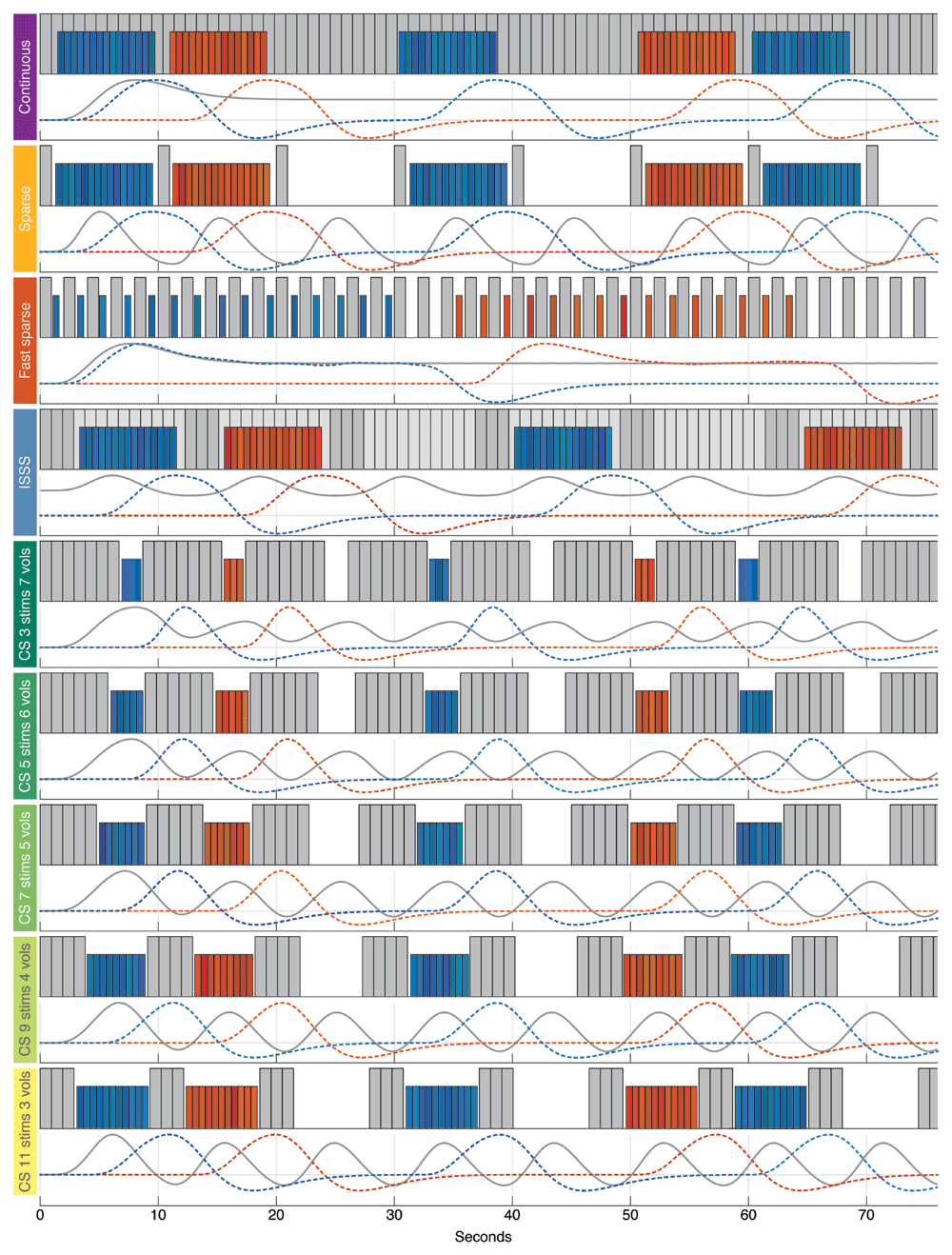
Figure 1. Schematic representation of all sequences and their associated hemodynamic response time courses.
[Each gray bar represents an acquisition volume (light gray bars are ISSS silent slice-selective excitation pulses). Each colored bar represents a sound stimulus (blue for one category, red for the other). Evoked hemodynamic responses to scanner noise and to sound stimuli are depicted at the bottom of each sequence, using the same color codes. CS, Clustered Sparse. For each clustered sparse sequence, the specific number of stimuli within a block and the number of acquisition volumes per cluster are specified.].
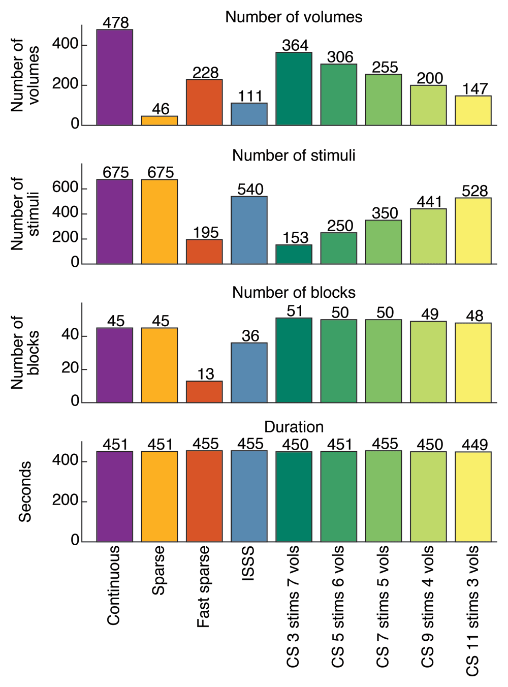
Figure 2. Sequence specifications.
Comparison of the number of volumes acquired, the number of stimuli presented, the number of blocks of stimuli presented and the total duration of each sequence (CS, Clustered Sparse).
Continuous. During the continuous sequence, scans were continuously collected (TR = TA, flip angle = 65°) while blocks of 15 stimuli (block duration = 8.2 s, inter-stimulus interval (ISI) = 50 ms) were presented alongside volume acquisitions. The time interval between two consecutive blocks was randomly jittered from 1 s to 2.5 s. This sequence allowed the acquisition of 478 volumes in 451 s and the presentation of 675 stimuli in 45 blocks.
Sparse. During sparse sampling, blocks of 15 stimuli (block duration = 8.2 s, ISI = 50 ms) were presented in between each volume acquisition (TR = 10 s, flip angle = 90°, silent period = 9.055 s). The gap between the end of a volume acquisition and the onset of sound stimulation was randomly jittered from 200 ms to 500 ms. This sequence allowed the acquisition of 46 volumes in 451 s and the presentation of 675 stimuli in 45 blocks.
Fast sparse. The fast sparse sampling sequence had a TR of 2 s (flip angle = 90°), leaving 1.055 s of silence between two acquisitions, during which a stimulus could be presented. The time interval between the end of a volume acquisition and the onset of a stimulus was randomly jittered from 100 ms to 400 ms. Thus, a block of 15 stimuli was approximately 15 TRs long (~30 s). Blocks of stimuli were randomly separated by either 2 or 3 TRs. This sequence allowed the acquisition of 228 volumes in 455 s and the presentation of 195 stimuli in 13 blocks.
ISSS. During the ISSS sequence, silent slice-selective excitation pulses were applied continuously for 10 TAs (quiet period = 9.45 s), followed by the acquisition of a cluster of 3 volumes (TR = TA, flip angle = 65°). The gap between the end of an acquisition cluster and the beginning of a block of stimuli (block duration = 8.2 s, ISI = 50 ms) was randomly jittered from 200 ms to 500 ms. This sequence allowed the acquisition of 111 volumes in 455 s and the presentation of 540 stimuli in 36 blocks.
Clustered sparse. Five variations of the clustered sparse sequence, with different block sizes and cluster sizes, were tested. For all variations, the following parameters were kept constant: ISI = 50 ms; the time interval between the end of an acquisition cluster and the start of a block of stimuli was randomly jittered from 100 ms to 300 ms; the TR within a cluster was 955 ms (10 ms more than the TA, to allow the scanner to listen to the volume acquisition trigger sent by the TDT RM1; flip angle = 60°).
Variations in the number of stimuli within a block were 3, 5, 7, 9 or 11, followed by an acquisition cluster of 7, 6, 5, 4 or 3 volumes, respectively. These sequences allowed the acquisition of 364, 306, 255, 200 or 147 volumes in 450, 451, 455, 450 or 449 s and the presentation of 153, 250, 350, 441 or 528 stimuli in 51, 50, 50, 49 or 48 blocks, respectively.
fMRI data analysis
Tissue segmentation and brain extraction were performed on the structural images using SPM's default segmentation procedure. Additionally, white matter and cerebrospinal fluid masks were eroded using a 3 mm cubic kernel in order to provide a mask that contains no region of interest to a principal component analysis of the functional data (see next paragraph). Transformation matrices between functional, anatomical and template volumes were computed using non-linear registration (ANTS, SyN). These transformation matrices were used to register the tissues segmentation to the functional data as well as to register the functional results to individual high-resolution anatomical scans and to the MNI152 ICBM 2009c Nonlinear Asymmetric template (Fonov et al., 2011). Functional data pre-processing included motion correction and spatial smoothing with a full-width half-maximum 3-dimensional Gaussian kernel that was twice the size of the functional voxels (i.e., 5 mm).
General linear model (GLM) estimates of responses to all sounds versus silence (“Sound vs. Silence” contrast) and to human voices against other sounds (“Human vs. Others” contrast) were computed with fMRISTAT (Worsley et al., 2002) using a hemodynamic response function modeled as the difference of two gamma density functions (Glover, 1999) with a peak at 5 s and an undershoot at 10 s. For all the sequences, the GLM included motion parameters (translations and rotations) as covariates of no interest. For the clustered sparse sequences, the first two principal components of a principal component analysis performed on the eroded mask of the functional voxels identified as containing white matter and cerebrospinal fluid were added as covariates of no interest to the GLM. Voxel significance was assessed by thresholding t-maps at p < 0.05, corrected for multiple comparisons using Gaussian Random Field Theory (Worsley et al., 1996). Spatial extent of significant voxels was computed for each sequence and contrast.
Maximum t-value is reported for three sets of ROIs: primary auditory cortex (A1), temporal voice areas (TVAs) and frontal voice areas (FVAs). In each subject and hemisphere, the A1 ROI contained the voxels of the probabilistic map (non-linearly registered to each subject functional space) of Heschl’s gyri provided with the MNI152 template (Penhune et al., 1996) that were above a probability of 0.3. TVAs and FVAs were sphere of 5 mm radius around the average ROI coordinates provided by (Aglieri et al., 2018). ROI locations are represented on Figure 3.
Fixed-effects group t-maps of both contrasts were computed using the template registered data from the two participants who were tested with all the protocols.
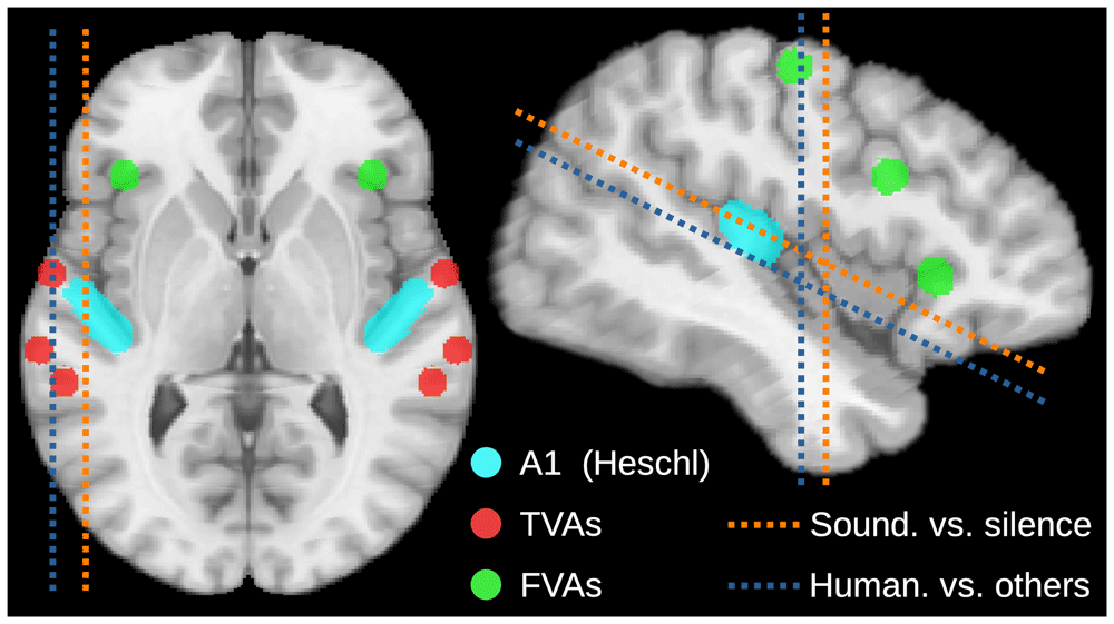
Figure 3. ROI and slice locations.
Location and angle of axial, sagittal and coronal slices shown on Figure 4 (dotted lines). Location of the ROIs at which max-t value is extracted and shown on Figure 5 (colored areas).
Results
Group results
Group results showed sound-related activation in response to all sounds of the voice localizer (“Sound vs. Silence” contrast) in all imaging protocols (Figure 4A). Auditory activation was found bilaterally in Heschl's gyrus, planum temporale and wider regions along the superior temporal gyrus and sulcus (STG and STS). Substantial activation was also found in the prefrontal cortex around the FVAs.
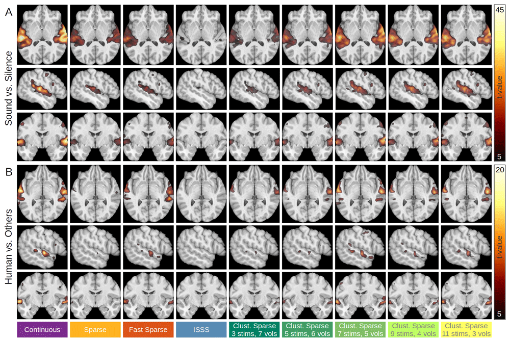
Figure 4. Group-averaged brain activations for all imaging sequences.
(A) “Sound vs. Silence” contrast. (B) “Human vs. Others” contrast. Slice locations for each contrast are represented on Figure 3.
Activations in response to human voices against other sounds (“Human vs. Others” contrast) were observed at typical TVA locations, along the STS and STG, for all imaging protocols except ISSS, and were also observed in the FVAs, for the continuous and clustered sparse sequences presenting five or more stimuli per trial (Figure 4B).
For both contrasts, the loci of maximal activation were very consistent from one imaging sequence to the other.
“Sound vs. Silence” individual results
Individual results for spatial extent and ROI maximum t-value are shown in Figure 5. On average, the continuous sequence showed larger spatial extent and greater maximum t-value than the other imaging sequences for the “Sound vs. Silence” contrast (Figure 5A). Continuous imaging performed better than sparse, fast sparse and ISSS for all three participants in both spatial extent and maximum t-value.
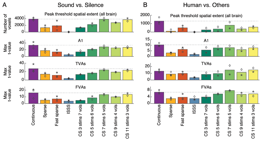
Figure 5. Spatial extent and ROI max t-values.
For the “Sound vs. Silence” (A) and the “Human vs. Others” (B) contrasts. Each bar represents the spatial extent or maximum t-value observed for a particular sequence and averaged across participants. Individual values are represented by symbols (square, diamond or star). To facilitate the comparison with the other sequences, the horizontal dotted line indicates the average value obtained using the continuous scanning sequence. CS, Clustered Sparse. ROI locations are represented on Figure 3.
The clustered sparse sequence, set to present seven stimuli per trial and acquire five volumes per cluster, showed the highest and largest auditory activation among the protocols that presented stimuli in silence (sparse, fast sparse, clustered sparse) or during reduced scanner noise (ISSS). Its average results approach those obtained with the continuous sequence (Figure 5A), and it shared best results with continuous scanning for the two participants who were tested with all the protocols.
Using ISSS, auditory activation barely reached significance in all three participants and maximum t-values were about one-sixth of those obtained with the continuous sequence (Figure 5A). ISSS always performed the worst, except for the FVAs maximum t-value in one participant.
Average spatial extents and maximum t-values obtained with the sparse and fast sparse sequences are about half of those obtained with the continuous sequence (Figure 5A). Results for two sequences were consistently in between those of continuous and ISSS for all three participants.
“Human vs. Others” individual results
The “Human vs. Others” contrast produced comparable but slightly different patterns (Figure 5B). In particular, the fast sparse sequence consistently outperformed the sparse sequence for this contrast, especially in terms of average spatial extent which was markedly higher. In TVAs and FVAs, the average maximum t-value was slightly higher for the clustered sparse sequence, which was set to present seven stimuli per trial and acquire five volumes per cluster, than for the continuous sequence. Both sequences yielded the best results for the two participants who were tested with all the protocols.
Discussion
We compared the performance of five different fMRI protocols of the same duration at detecting auditory and voice-related activation in human participants adequately protected from scanner noise. Under these conditions, continuous imaging was found to provide the best results, closely followed by a clustered sparse sequence in which stimulus and acquisition durations were both set to be around 4 s. Sparse and fast sparse sampling provided intermediate results, while ISSS showed the poorest performance.
The superior results of continuous imaging align with previous duration-matched comparisons between continuous and sparse sampling protocols, and can be explained by the combination of its established strength in maximizing data acquisition and the good protection from scanner noise provided by contemporary equipment. However, in setups where optimal protection from the scanner noise cannot be achieved, or where the magnetic field is higher, resulting in increased scanner noise (Akbar et al., 2023), the observed superiority of continuous imaging performance may be compromised, while that of the protocols presenting stimuli during silence may not. In such setups, or when the experimental design necessitates the presentation of stimuli in silence, a clustered sparse sequence with the appropriate parameters may be the optimal choice. Prior work using clustered sparse imaging has demonstrated that it can outperform continuous scanning in certain contexts (Schmidt et al., 2008), and the present study likewise showed that its performance approached that of continuous scanning. Additionally, we show that T1 signal decay can be readily corrected by adding the first two principal components of a PCA performed on the white matter tissue as nuisance regressors to the linear model.
Fast sparse sampling, with the advantage of constant TRs and longitudinal magnetization maintained at a steady state, also showed promising results, especially for the "Human vs. Others" contrast. For this sequence, we presented the same number of stimuli per block as for the continuous and sparse sequences, resulting in much longer blocks in comparison. In this particular design, fewer blocks could be presented in the fixed duration of a run, to the detriment of the sequence. Comparing variations of the fast sparse sequence, as we did for the clustered sparse sequence, would shed light on the optimal parameters for block duration and improve the performance of this sequence. However, because the stimuli are quickly interleaved with volume acquisitions, fast sparse sampling is only suitable for short stimuli, limiting its generalizability to tasks involving longer sounds.
The original method that allows stimuli to be presented in silence, sparse sampling, produced results that were about half those of clustered sparse and continuous imaging. This highlights the main limitation of this method, its low data sampling per unit of time. However, If sparse does not seem to be the optimal sequence choice for a voice localizer, it may be crucial for certain study designs to separate acquisitions by a long enough interval to ensure that the hemodynamic response to the previous acquisition noise has passed. In such cases, our clustered sparse results suggest that it may be appropriate to cluster multiple volumes instead of acquiring volumes one after the other.
The results obtained with ISSS gave the lowest activation results of all the acquisition schemes. We have reservations about these results as they are very different from previous comparisons of ISSS with continuous or sparse sequences. As a side note, participants perceived the pseudo-silent periods of ISSS as moderately less loud than the acquisition periods. The ISSS sequence used in this study was obtained from the CMRR multiband sequence, version R016a. In the current version (R017), the implementation of ISSS is described as providing quieter "silent" periods.
A key limitation of this study is the small sample size of only three participants, which restricts the generalizability of the findings. However, clear trends were observed and sequences were ranked in a consistent manner across participants, suggesting that the overall picture appears to be valid. Furthermore, this study employed a block design, and it remains an open question as to which protocol would perform best in an event-related design.
In summary, continuous imaging is a powerful tool for auditory fMRI, especially in designs in which scanner noise masking does not significantly alter categorical perception and when human subjects are well protected from scanner noise. However, when stimuli must be presented in silence, clustered sparse sampling, with its specific balance between stimulation and acquisition time, emerges as a more effective protocol.
Ethics and consent
Participants gave written informed consent and were not paid for their participation. The experiment was granted ethical approval by Aix-Marseille Université “Comité Protection des Personnes”—“Committee for the Protection of Individuals”: CPP 2017-A03614–49, February 13, 2019. The experimental procedures conformed to the World Medical Association’s Declaration of Helsinki.









