Introduction
The Foodlevers project
The Foodlevers project, conducted from 2020 to 2023, aimed to identify leverage points for enhancing and scaling organic and sustainable food systems in Europe [Davelaar, 2021; Urmetzer et al., 2020]. The project targeted three primary realms: reconnecting people to a nature friendly behaviour, restructuring institutions through policy makers informed choices, and rethinking food-related knowledge at producers and consumers level. By examining case studies across seven European countries (Belgium, Finland, Germany, Italy, Poland, Romania and United Kingdom), it assessed innovative food systems' sustainability and developed scenarios for systematic transformation.
Key methods of the Foodlevers project included holistic sustainability assessments [Dorninger et al., 2020] and stakeholder-driven decision-making models using FCM. The project emphasised addressing root causes of unsustainability and explored how behaviour, institutional frameworks, and market dynamics contribute to transformative opportunities. Its findings provide insights into strategies for accelerating sustainability transitions in food production and consumption.
FCMs are qualitative models of systems based on variables and their causal relationships, translated into semi-quantitative graphs. Foodlevers applied FCM in all the participant countries, gathering the stakeholders in dedicated workshops. Stakeholders defined system variables and their causal links, and scenarios of change influenced by external drivers. Outputs included maps analysed for insights into system dynamics. The maps were then simplified, retaining only the most significant variables, producing the synthesis maps object of the proposed study. These models provided structured insights into the European food-related complex systems, fostering sustainability in complex European food systems.
While previous analysis within the Foodlevers project explored the construction and interpretation of FCMs [Foodlevers, 2023], this article shifts focus towards the comparative analysis of network structures. Specifically, it examines how the connections between variables differ across countries’ case studies. The methodology emphasises the quantitative and qualitative comparison of network characteristics, including link density, strength distribution, and the role of key variables.
Fuzzy cognitive mapping in agricultural policy
Fuzzy Logic is a non-binary logic, which allows for reasoning and decision-making under uncertainty [Zadeh, 1965]. Unlike binary logic, where statements are either true or false, fuzzy logic incorporates the typical grey areas reasoning of real-world problems. In fuzzy logic, variables assume a degree of truth, conventionally represented by a continuum between 0 and 1. In the content of fuzzy decision making, as is the case of our study, the degree of truth can be interpreted as a score or importance, emerging from the causal network [Kahraman, 2008; Zadeh, 1975].
Cognitive Mapping allows a group of individuals to express their knowledge of a subject through a conceptual, graphical representation made of nodes (i.e concepts) and links (i.e. causal relations), without explicitly recurring to quantitative mathematical techniques. Cognitive Mapping is particularly useful for identifying decision-making processes in complex systems like the ones object of the Foodlevers project.
Fuzzy Cognitive Mapping, a qualitative modeling technique used for analysing complex systems, was first introduced by Kosko as an extension of cognitive mapping, exploiting the techniques of fuzzy logic [Kosko, 1986]. FCM represents complex systems as networks of interconnected concepts, where the nodes are variables or factors, and the edges, usually represented as arrows, indicate causal relationships [Kosko, 1988].
FCM techniques have been successfully applied in the field of agricultural policy and stakeholders’ perceptions in Europe, with notable examples from Austria [Targetti et al., 2021], Denmark [Averbuch et al., 2022], Italy [Pisanelli et al., 2023] and Spain [Martinez et al., 2018], and in Turkey [Özesmi & Özesmi, 2003]. The goal of the present study is to compare stakeholders' perceptions across several European countries regarding the promotion of organic and sustainable farming [Eyhorn et al., 2019; Reganold & Wachter, 2016] as well as land use management [Willett et al., 2019]. This comparison is based on data collected by the Foodlevers project partners. The single countries FCM analysis is available on the project’s resources site [Foodlevers, 2023].
Methods
Data collection and selection
The input material for this study consists of a set of relevant concepts (the variables) interconnected through a network of causal relationships (the weights). This material was collected during workshops conducted in 2002 as part of the Foodlevers project in Belgium, Finland, Germany, Italy, Poland, Romania, and the United Kingdom, organising discussion panels of farmers, advisors, researchers and policy makers [Khan & Quaddus, 2004; Staton et al., 2024b]. With the goal of providing variables and weights, the data collection process followed different strategies. Some partners used stickers, coloured pencils and paper, while others utilised assisted graphical web tools. Regardless of the method, the final product for each country consisted of a list of variables and a matrix of weights, arranged as a network map, according to the principles of FCM [Felix et al., 2019; Gray et al., 2014; Kahraman, 2008].
Conventionally, variables are represented as nodes of a graph, while causal relationships are depicted as directed arrows pointing from the causing node to the affected node. Each arrow carries a weight in the range (0,1] for a positive direct influence or [-1,0) for an inverse influence. Self-interactions are not permitted but mutual interactions are (Figure 1).
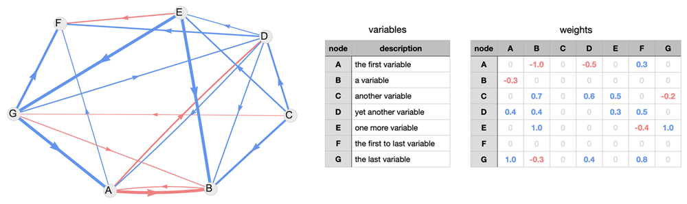
Figure 1. A Fuzzy Cognitive Map network and the corresponding variables and weight matrix.
Conventionally, the arrows in an FCM graph have a thickness proportional to the intensity (i.e., the absolute value of the weight) and are often coloured to represent the type of relationship. In our case, we use blue for direct relationships and red for inverse ones.
The set of nodes {Ni} is connected through weights Wi,j, where the first index corresponds to the originating node (row index of Figure 1) and the second to the receiving node (column index). The nodes without incoming arrows are called drivers and those without outgoing arrows are called receivers. For each node, we evaluated the commonly used metrics [Felix et al., 2019; Özesmi & Özesmi, 2004], in order to find the most important variables:
ent Ni = number of arrows entering node Ni. the drivers are {Nk | ent Nk = 0}.
ext Ni = number of arrows exiting node Ni. the receivers are {Nk | ext Nk = 0}.
ord Ni = ent Ni + ext Ni is the order of node Ni
id is the indegree of node Ni
od is the oudegree of node Ni
deg Ni = id Ni + od Ni is the degree of node Ni
All the mentioned metrics are available in the published data [Foodlevers, 2023; Staton et al., 2024b]. The synthesis variables are shown below in each of the country dedicated sections.
The order and degree of a node are often related: the order simply counts the number of connecting edges, while the degree (also referred to as centrality in the literature) considers the intensity of the connections, regardless of whether they are direct or inverse, incoming or outgoing. The degree of a node is recognised as the most appropriate indicator of a node's importance [Özesmi & Özesmi, 2004]. To identify the most representative variables among those provided in each country’s original set, we evaluated the degree distribution and assigned scores based on quartiles [Felix et al., 2019]. We then selected the variables in the third and fourth quartiles, resulting in comparable sets of 12 to 16 variables per country, with the exception of Poland, where all 9 of the original variables were included. The full original sets of variables can be found in the Foodlevers project documentation [Foodlevers, 2023].
Network evolution
We employed a double-distilled strategy: first, we identified the most important concepts from each country's FCM, and then refined these further by selecting the highest-value concepts using statistical ensembles and fuzzy dynamics techniques, ensuring a robust and focused analysis of sustainability priorities.
The concept behind FCM evaluation is that, starting from an initial set of values assigned to the nodes, the causal relationships between the nodes are iteratively updated using a recursive application of an evolution function. This process simulates how changes in one variable (node) influence others over time, ultimately (hopefully) converging to a stable state based on the system's dynamics. Said the initial conditions, i.e. the starting values of nodes the values at kth evolution step are given by
where α ∈ [0,1] weights the resistance of the initial previous value, F is the so-called activation function, it could be a sigmoid, a rescaled inverse tangent or hyperbolic tangent, or whatever keeps the values smoothly and monotonically inside [0,1]. We conducted the network analysis in R environment, exploiting R’s fcm package functions [Dikopoulou & Papageorgiou, 2022], using a sigmoid activation function
The λ parameter controls the sigmoid function steepness [Glykas, 2010; Özesmi & Özesmi, 2004]. Given the highly interconnected nature of relationships in the network, despite the dampening effect of the sigmoid (which ensures values remain within the [0, 1] range), convergence is not guaranteed [Alizadeh & Ghazanfari, 2009; Kottas et al., 2007; Liang & Zhu, 2024; Tsadiras, 2008; Wang et al., 1990]. Three possible outcomes are observed in such systems:
Equilibrium: The node values reach a steady state, eventually stabilising within a given tolerance.
Periodic behaviour: After an initial transient phase, the node values exhibit periodic oscillations, returning multiple times to the same sequence of values.
Chaotic behaviour: The node values fluctuate irregularly, without any apparent periodicity or convergence.
In our analysis, we heuristically observed that all the networks corresponding to the countries studied reached a steady state rapidly, using λ =1. Other values of the parameter λ gave comparable results.
We used both evolution rules of Equation (2), obtaining the same results in terms of variables ranking, with consistently higher values obtained with Equation (2b) with respect to Equation (2a).
Despite the fact that drivers, by definition, have no incoming arrows, their values are not left untouched by Equations (2). On the contrary, their values quickly reach 0.5 using Equation (2a), approaching (1 + e0)−1 from the first iteration, as can be seen in Figure 2, variable C. This loss of memory of the initial value reflects their lack of influence from other nodes in the network. The value 0.5 is an artefact due to the uniform random distribution of initial conditions. The initial value of receivers is scarcely relevant as well, as the application of Equations (2) determines their effective value.
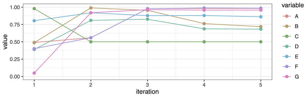
Figure 2. The equikibrium values of the network in Figure 1 (right end), given random initial values (left).
Although setting different initial values could, in principle, lead to varying outcomes, our ensemble analysis focused on the network values consistently revealed a stable equilibrium across all our case studies.
Ensemble analysis
For each country, we performed an ensemble analysis consisting of thousands of reproductions of the same network (i.e., the weights remained fixed) with different random initial conditions . The initial values were drawn from a random uniform distribution in the range [0, 1], irrespective of their semantic meaning [Contucci & Vernia, 2020; Durlauf, 1999]. This approach allowed us to focus purely on the network's structural dynamics without considering the specific interpretations of what the nodes represent. In detail, we ran 10000 simulations for each country, limiting the number of iterations to 2, 3, 4, 5, and 10, resulting in a total of 50000 ensemble elements per country. For each ensemble, we analysed the relationship between the final and initial conditions to assess the network's behaviour under varying dynamics, calculating the variability of the nodes values at each iteration as the equilibrium is approached.
To quantify the convergence to equilibrium we compared the shrinking of the values range at the kth iteration, finding an inverse exponential range decrease. Very few outliers were found (a few units per country ensemble), corresponding to extremely unlikely initial values clustered about 0 or 1. As shown in Figure 3, the network dynamics can be captured by juxtaposing the ranges at 2, 3, 4, 5, and 10 iterations for each variable. In some cases, the equilibrium (tracked using the distribution median) is approached monotonically. However, this is not always the case; not surprisingly, most often the higher values are approached from below, while the lower values are reached from above. This is a signature of the smoothness of the sigmoid function in Equations (2). The equilibrium was reached, in most cases, between 5 and 10 iterations, within a tolerance of 0.001. All the detailed ensemble dynamics plots can be found in the published data.
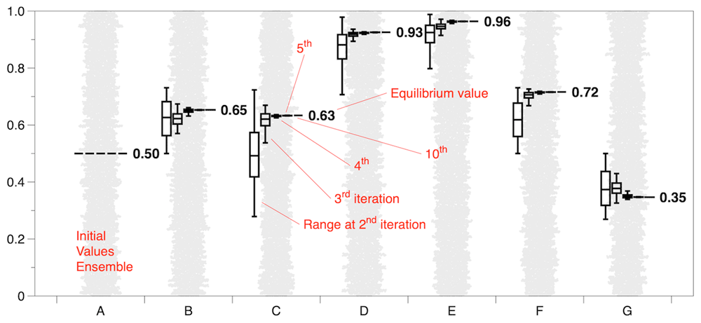
Figure 3. A fictiomal FCM example of initial distribution (grey cloud) end equilibrum values approaching (box plots).
The ensembles from the different case studies exhibit similar behaviour in approaching equilibrium. To quantify the rate at which equilibrium is reached, we performed a negative-exponential regression analysis of the variable value ranges against the maximum number of iterations, Equation (3), yielding comparable results across the case studies.
We found k values ranging from 0.45 (Germany) to 0.77 (UK), with R2 values exceeding 0.8, except for Germany, where R2 is 0.77. The overall regression (i.e., for all countries combined) yields k = 0.67 with R2 = 0.8. The aforementioned k values result in a halving time, k ln 2, which is roughly 0.5. This means that each iteration reduces the range by about one-quarter of the previous range, leading to rapid convergence.
Figure 4 shows the overall dynamics regression for the cumulative case. The single countries regressions can be found in the published data.
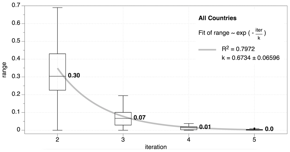
Figure 4. The behaviour of values distribution vs iterations number, Equation (3).
Graphs topological analysis
Geometrically speaking, a FCM is a graph G made of nodes and connections: G = ({Ni}, {wij}). In order to characterise the FCMs, we use the number of nodes n = #{Ni}, drivers nd = #{Ni|entNi = 0}, receivers nr = #{Ni | ext Ni = 0}, and the number of edges m = #{wi,j | wi,j ≠ 0 or, equivalently m = ∑i,j θ(|wi,j|) where θ(⋅) is the Heaviside step function. Following [Glykas, 2010; Özesmi & Özesmi, 2004], we derive some indices: the density
and the complexity
of
G. The density
d is the ratio of the actual over the maximum possible connections (
wii = 0), it measures how saturated is a given graph. The complexity values range from 0 (no receivers) to infinity (no drivers). A low complexity suggests a drivers-dominated network, with a sort of cascading effect, while a high complexity suggests a certain freedom for the receivers. We attributed the value 1 to the indeterminate 0/0 case, when
nd =
nr = 0, indicating that neither drivers nor receivers prevail. A further graph index is the hierarchy of
G, evaluated from the graph’s outgoing connections:
The hierarchy goes from 0, a so-called fully democratic graph, to 1, a purely hierarchical graph. The graph’s h characterises the level of organisation of the system represented by G. We found h values ranging from 0.07 for Poland to 0.49 for UK. in general, c, d and h should not be correlated, as it is in our case, with |r| < 0.1 for h~c and h~d, see Figure 5, left.
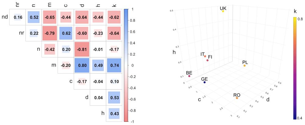
Figure 5. Left: pairwise Pearson correlation coefficients.
Right: k values in (c,d,h) space.
The convergence rate k is positively strongly correlated with m, correlated with d and h, and negatively correlated with both nd and nr. Since c is correlated with nd and nr, and d is strongly correlated with n and m, we will use only complexity, density and hierarchy as topological indices for our case studies.
The countries graphs are sparsely distributed in the (c, d, h) space, as shown in Figure 5. Finland and Italy form the only cluster with very close indices values. United Kingdom is far from all the other countries.
Results
In the following sections, a detailed analysis will be provided for each country involved in the study. For each country, a table of variables and a graphical representation of its FCM will be presented to highlight the system’s structure and dynamics. It is important to note, however, that the arrangement of nodes in the maps is arbitrary and does not imply any specific spatial or hierarchical relationships among the variables. To fully engage with the intricacies of these FCMs, readers are strongly encouraged to explore the accompanying interactive HTML pages, available in the designated data repository. These interactive maps allow for a more dynamic view of the system’s structure, allowing to investigate connections, weights, and relationships in greater depth, offering insights beyond the static visualisations presented here. The detailed ensemble dynamics is also available in said repository.
Table 1 presents a summary of the indices calculated for each country, with a particular focus on density d, hierarchy h, and complexity c, as these indices are independent of the total number of variables and therefore provide a consistent basis for cross-country comparisons. The other metrics include the number of variables n, drivers nd, receivers nr, and number of connections m. We also show the ensemble convergence rate k, from Equation (3).
Table 1. Relevant measures of the Foodlevers countries’ FCMs.
| Country | n | nd | nr | m | d | c | h | k |
|---|
| Belgium | 16 | 5 | 0 | 37 | 0.15 | 0.00 | 0.09 | 0.63 |
| Finland | 14 | 1 | 1 | 45 | 0.25 | 1.00 | 0.23 | 0.65 |
| Germany | 13 | 3 | 4 | 18 | 0.12 | 1.33 | 0.13 | 0.45 |
| Italy | 12 | 2 | 2 | 29 | 0.22 | 1.00 | 0.26 | 0.69 |
| Poland | 9 | 0 | 0 | 68 | 0.94 | 1.00 | 0.07 | 0.73 |
| Romania | 16 | 1 | 3 | 33 | 0.14 | 3.00 | 0.14 | 0.71 |
| UK | 13 | 0 | 0 | 79 | 0.51 | 1.00 | 0.49 | 0.77 |
A high density fuzzy cognitive map indicates a system where variables are heavily interconnected, suggesting a rich and intricate web of influences. Conversely, lower density implies a sparser map with fewer connections, potentially simplifying the system’s dynamics. Poland exhibits an outstandingly high density (0.94 i.e. close to saturation) and UK exhibits a relatively high density, indicating highly interconnected systems. This complexity likely stems from a need to represent diverse stakeholder inputs (Poland) and intricate system dynamics (UK), such as market forces and policy impacts. Belgium, Germany and Romania, on the other hand, have lower densities, signalling simpler structures that might focus on a narrower set of relationships, prioritising key drivers and outcomes. Finland and Italy fall in the mid-range, suggesting a balanced representation of the system. High-density maps are excellent for exploring detailed causal pathways, possibly highlighting inner structures, but may risk overcomplicating interpretations. Low-density maps, while less informative, easily point out core dynamics and so leverage points (Table 1).
A high hierarchy h suggests a strongly hierarchical system dominated by a few key variables leading the network dynamics (not necessarily drivers), while a low index points to a more distributed influence pattern, in fact, Equation (6) highlights the presence of nodes of distinguished outdegree with respect to the average. UK has a notably high hierarchy, reflecting a network structure where a few key variables drive most of the outcomes. This can indicate a focus on specific policy levers and environmental factors as primary influencers. Finland and Italy show intermediate levels of hierarchy, balancing centralised and distributed influences. Germany and Romania have lower hierarchy, representing more egalitarian systems where influence is distributed across many variables, better capturing the interdependence of factors. Belgium and Poland show the lowest h values, suggesting even more distributed influences among the variables, especially in the case of Poland. Higher hierarchical systems may facilitate targeted interventions but risk oversimplification, while lower hierarchical systems provide richer feedback loops at the cost of interpretive clarity.
Complexity c quantifies the interplay between drivers and receivers, offering insight into the system’s feedback dynamics. The name complexity is somehow misleading, not being related to the intricacy of the network, but to the drivers and receivers alone. Higher complexity values indicate straightforward interdependencies, while lower values suggest less linear, one-way causal chains. Poland and UK maps have no drivers and no receivers, they have been conventionally assigned c = 1. Romania stands out with the highest complexity, reflecting a somehow linear dynamic system, without deeply interlinked nodes. This likely mirrors the challenges of addressing multifaceted issues such as education, bureaucracy, and market dynamics. On the other hand, Belgium shows c = 0, having many drivers but no receivers at all. Finland, Germany and Italy have a balanced c around 1.
The k values, representing the variables’ rate of convergence towards equilibrium, show noticeable variations across countries, offering insights into the dynamism of their respective systems. Higher k values (UK at 0.77, Poland at 0.73, and Romania at 0.71) suggest that these systems exhibit faster convergence towards equilibrium. This implies that changes within these systems stabilise more quickly, potentially reflecting more direct or less complex feedback mechanisms. The intermediate values seen in Belgium (0.63), Finland (0.65), and Italy (0.69) indicate systems that balance these dynamics, with moderate rates of stabilisation. In contrast, lower k values (Germany at 0.45) indicate slower convergence, suggesting that the system may experience prolonged transitions before reaching equilibrium, despite the low density (d = 0.12). This could be a sign of delayed responses between variables, possibly due to low relationships weights. Generally speaking, these differences highlight variations in system responsiveness across countries, potentially influenced by the nature of their variables, feedback loops, and the degree of interconnectedness. Such information is crucial for tailoring interventions and predicting system behaviour under external changes.
For each country, we evaluated the quartiles of the distribution of the variables’ values to identify key patterns within the system. This approach allows for a structured analysis of the variables based on their relative influence. In particular, we will focus on discussing the variables that fall into the fourth quartile, as they represent the most important and influential nodes within each FCM. These high-value variables typically play a central role in driving system dynamics, acting as pivoting leverage points or indicators of key system behaviours. By highlighting these influential nodes, we aim to provide deeper insights into the structural and functional characteristics of each country’s FCM.
The FCMs are presented as tables of variables accompanied by their respective attributes and as graphs where relationships are visualised with edge thickness representing the intensity of the connection and edge colour indicating its character, blue for direct and red for inverse relationships. For each variable, the following attributes are included in the table:
node - the variable label A, B, C… as it appears on the map, corresponding the actual realisation of the abstract {Ni} set,
value - the variable’s equilibrium value,
rank - the rank of the variable based on its equilibrium value,
ent - the number incoming arrows,
ext - the number of outgoing arrows,
ord - the node order,
id - the node indegree,
od - the node outdegree,
deg the node degree,
quart - the quartile to which the variable’s equilibrium value belongs, Q1 to Q4,
variable description - the textual explanation of the variable, as recorded verbatim during the stakeholders' workshops.
The metrics of the maps are summarised in Table 1.
Belgium
The variables for Belgium’s FCM (Figure 6) are detailed in Table 2. Among these, the most relevant variables—those in the fourth quartile—are particularly noteworthy for their influence on the system’s dynamics. These include: G Consumer demand (market size), which reflects the size of the market driven by consumer behaviour; N Sector size (volume of organic market), indicating the overall scale of the organic sector; I Society’s/consumers’ awareness about organic, capturing public awareness and its impact; and K Number of converted/started (innovative) organic farms, representing the adoption and growth of innovative organic farming practices. These variables reflect the structure and function of Belgium’s organic market system. The weights in the Belgian FCM are distributed across a broad spectrum of values, indicating that the stakeholders’ workshop involved a comprehensive and detailed discussion. This wide-ranging distribution suggests that participants considered diverse aspects of the system, reflecting a thoughtful and inclusive deliberation process aimed at capturing the complexity of the organic market dynamics. The map reveals five drivers—A, B, C, D, and E—out of sixteen nodes. This notable proportion reflects an effort to achieve a comprehensive understanding of the key driving factors influencing organic farming, particularly those shaping market dynamics. Although these driver nodes have relatively low values due to the application of Equation (2a/b), they were explicitly selected by stakeholders as drivers and therefore hold significant importance in the system. The identified drivers include: Momentum in market - both positive (A) and negative (B), difference between existing and innovative farm model, and legal certainty (e.g., permits), and labor intensiveness (Table 2).
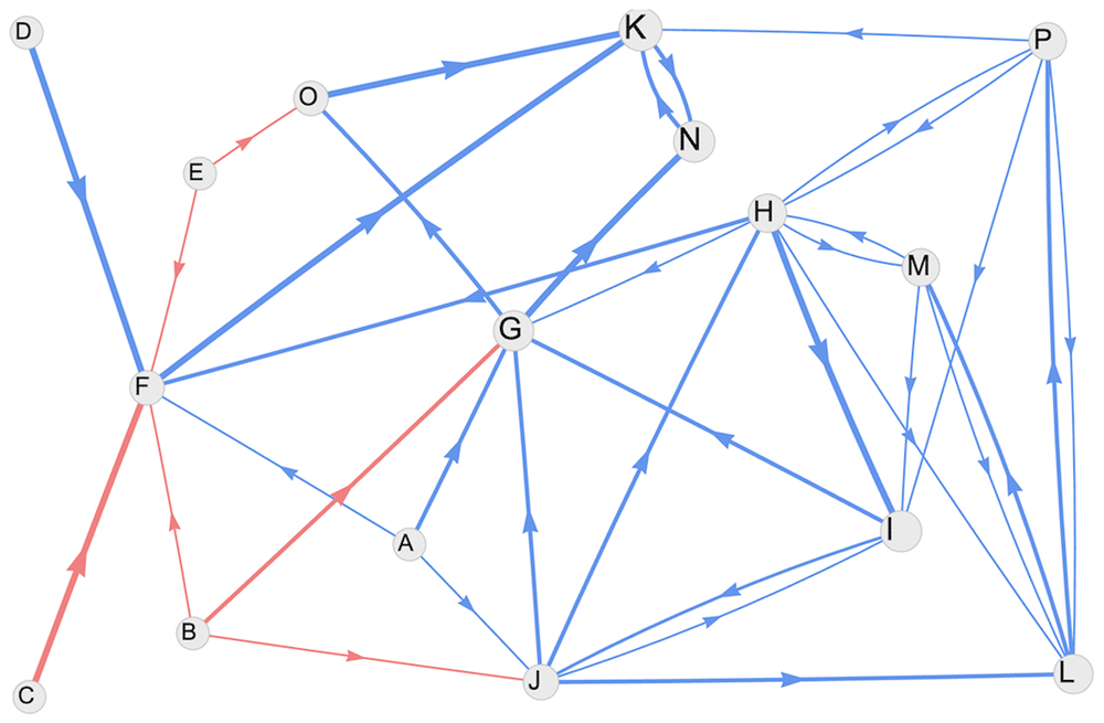
Figure 6. Belgian FCM graph.
Table 2. Belgian variables.
| Node | value | rank | ent | ext | ord | id | od | deg | quart | variable description |
|---|
| A | 0.500 | 12 | 0 | 3 | 3 | 0.00 | 1.32 | 1.32 | Q1 | Momentum in market – Crisis situation (pos), e.g. corona |
| B | 0.500 | 12 | 0 | 3 | 3 | 0.00 | 1.32 | 1.32 | Q1 | Momentum in market – Crisis situation (neg), e.g. inflation |
| C | 0.500 | 12 | 0 | 1 | 1 | 0.00 | 1.00 | 1.00 | Q1 | difference between existing farm model and innovative
organic model, e.g. in scale, existing buildings, etc |
| D | 0.500 | 12 | 0 | 1 | 1 | 0.00 | 1.00 | 1.00 | Q1 | legal certainty e.g. of permits |
| E | 0.500 | 12 | 0 | 2 | 2 | 0.00 | 0.66 | 0.66 | Q1 | labor intensiveness |
| F | 0.573 | 11 | 6 | 1 | 7 | 3.65 | 1.00 | 4.65 | Q2 | farmer’s own conviction/drive, ideological personality
farmers |
| G | 0.759 | 4 | 5 | 2 | 7 | 2.97 | 1.66 | 4.63 | Q4 | consumer demand (market size) |
| H | 0.698 | 6 | 3 | 6 | 9 | 1.32 | 2.98 | 4.30 | Q3 | Policy (makers) work supportive (of organic farming) |
| I | 0.792 | 2 | 4 | 2 | 6 | 1.99 | 1.16 | 3.15 | Q4 | Society’s/ consumers’ awareness about organic |
| J | 0.598 | 9 | 3 | 4 | 7 | 1.16 | 2.31 | 3.47 | Q2 | Mindset of consumers, Ideological personality consumers |
| K | 0.870 | 1 | 4 | 1 | 5 | 2.99 | 0.66 | 3.65 | Q4 | number of converted/started (innovative) organic farms |
| L | 0.744 | 5 | 4 | 2 | 6 | 1.65 | 1.32 | 2.97 | Q3 | Successful farms as examples |
| M | 0.673 | 8 | 2 | 3 | 5 | 0.99 | 0.99 | 1.98 | Q3 | Research, knowledge on benefits of organic vs non-organic |
| N | 0.791 | 3 | 2 | 1 | 3 | 1.66 | 0.66 | 2.32 | Q4 | Sector size (volume of organic market) |
| O | 0.583 | 10 | 2 | 1 | 3 | 0.99 | 1.00 | 1.99 | Q2 | profitability |
| P | 0.673 | 7 | 2 | 4 | 6 | 0.99 | 1.32 | 2.31 | Q3 | Practice research for organic farming |
The graph for Belgium’s FCM reveals the presence of numerous tightly connected pairs of mutually influencing variables, forming short feedback loops, e.g. I-J, L-P, H-M, K-N and L-M. These short-chain loops can amplify feedback effects within the system, leading to rapid changes and intensifications in variable states. Notably, this phenomenon occurs regardless of the intensity of the relationships, as long as the connections share the same character (either both direct or both inverse). Such structural features can drive quick system responses, underscoring the importance of these feedback mechanisms in shaping the dynamics of the Belgian organic market system. The graph density is quite sparse (d = 0.15, h = 0.09).
The key variables identified for Belgium reflect a system primarily concerned with the demand and supply aspects of the organic market, as well as societal awareness and adoption trends. However, it is notable that these variables lack representation of physical measures such as environmental conditions, resource use, or ecological impacts, which are often critical in assessing the broader sustainability of organic systems. The remarkable total of five drivers reflects an effort to achieve a comprehensive understanding of the key driving factors influencing organic farming, particularly those shaping the market dynamics.
The convergence rate of the network is k = 0.63, an average value in our study.
Finland
The Finnish FCM (Figure 7) is characterised by an intriguing structure where all connections are assigned weights of either +1 or -1. This lack of nuanced weighting suggests a simplified approach to representing relationships, where the direction of influence is captured without reflecting varying intensities. Despite this simplicity, the map includes a significant number of connections, resulting in a relatively high density of 0.25. This density highlights the interconnected nature of the system, with many variables influencing one another (Table 3).
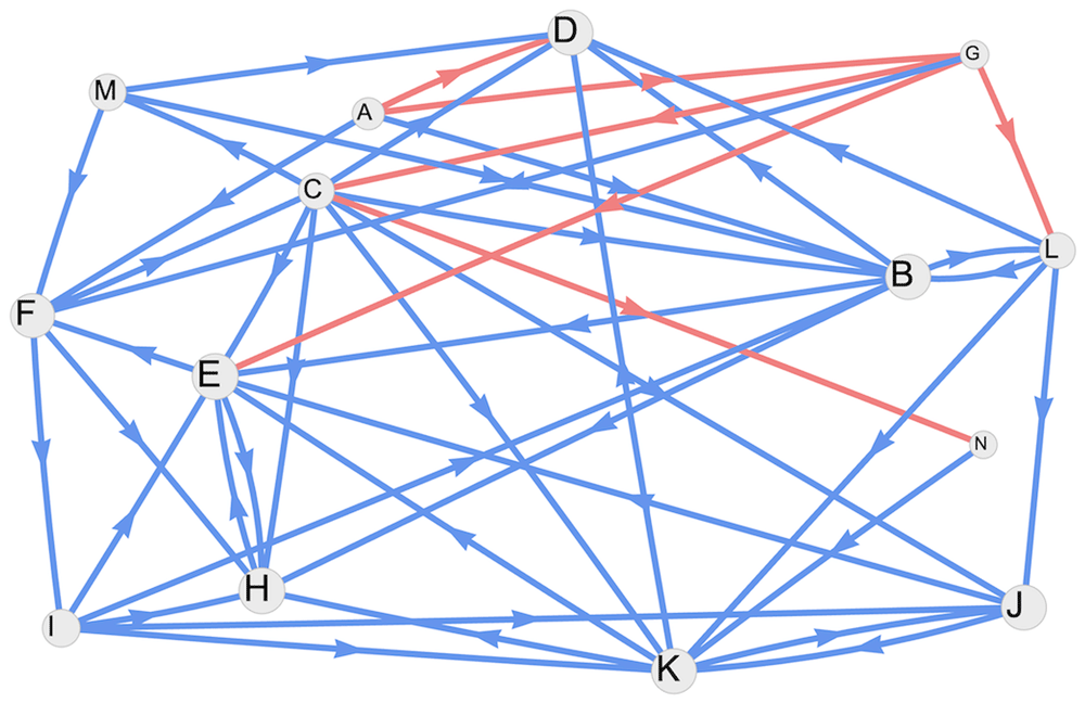
Figure 7. Finnish FCM graph.
Table 3. Finnish variables.
| node | value | rank | ent | ext | ord | id | od | deg | quart | variable description |
|---|
| A | 0.500 | 12 | 0 | 4 | 4 | 0.00 | 4.00 | 4.00 | Q1 | Increase in climate and weather risks |
| B | 0.959 | 5 | 5 | 4 | 9 | 5.00 | 4.00 | 9.00 | Q3 | Technological innovation in organic farming |
| C | 0.634 | 11 | 2 | 8 | 10 | 2.00 | 8.00 | 10.00 | Q1 | Education of organic food for students in different
disciplines, e.g. agriculture, forestry, retail, education |
| D | 0.966 | 3 | 6 | 0 | 6 | 6.00 | 0.00 | 6.00 | Q4 | Wellbeing of the producer values |
| E | 0.992 | 2 | 7 | 2 | 9 | 7.00 | 2.00 | 9.00 | Q4 | Media discourse on organic food, agriculture, climate |
| F | 0.926 | 7 | 4 | 3 | 7 | 4.00 | 3.00 | 7.00 | Q3 | Policies in a given time and a given place |
| G | 0.378 | 13 | 1 | 4 | 5 | 1.00 | 4.00 | 5.00 | Q1 | Conflicts and crises |
| H | 0.994 | 1 | 6 | 1 | 7 | 6.00 | 1.00 | 7.00 | Q4 | Visibility of organic farming in society |
| I | 0.716 | 8 | 1 | 5 | 6 | 1.00 | 5.00 | 6.00 | Q2 | Education of organic farming at all school levels |
| J | 0.951 | 6 | 4 | 2 | 6 | 4.00 | 2.00 | 6.00 | Q3 | Communities/networks/value ecosystems |
| K | 0.964 | 4 | 5 | 4 | 9 | 5.00 | 4.00 | 9.00 | Q4 | Farmers and entrepreneurs values |
| L | 0.641 | 10 | 2 | 4 | 6 | 2.00 | 4.00 | 6.00 | Q2 | Money /support for the production |
| M | 0.653 | 9 | 1 | 3 | 4 | 1.00 | 3.00 | 4.00 | Q2 | The need for social responsibility |
| N | 0.347 | 14 | 1 | 1 | 2 | 1.00 | 1.00 | 2.00 | Q1 | Monopoly on seeds and fertilizers, with increasing prices |
The variables in the fourth quartile—H Visibility of organic farming in society, E Media discourse on organic food, agriculture, and climate, D Wellbeing of the producer values, and K Farmers and entrepreneurs values—emerge as particularly influential within the system. These variables emphasise the societal and personal dimensions of organic farming, underscoring the importance of public awareness, media representation, and the values held by producers and entrepreneurs. Together, they highlight a stakeholder-driven perspective that prioritises the social and cultural aspects of Finland’s organic farming sector. The variables G Conflicts and crises and N Monopoly on seeds and fertilisers with increasing prices are notable for their low ensemble equilibrium values, indicating that, while present in the system, their overall influence within the Finnish FCM is comparatively limited.
It is noteworthy that node C Education of organic food for students in different disciplines, e.g., agriculture, forestry, retail, education, has a relatively low equilibrium value, yet its high degree establishes it as a pivotal element within the network. There are a few pairs of positively connected nodes—B-L, E-H, and K-J—that contribute significantly to the overall ensemble, reflected in the value of k = 0.65. The number of inverse relationships is low compared to direct ones, a pattern consistent with all the other countries in our study. Unsurprisingly, the variable with the most negative influence is G Conflicts and crises, which is perceived as a hindrance to the development of sustainable agriculture. In Finland, the FCM highlights a notable emphasis on the personal dimension of human connections between producers and consumers, while physical variables are not perceived as particularly crucial to the system. This focus reflects a stakeholder perspective that prioritises social and relational factors over environmental or resource-based considerations. Variables such as Wellbeing of the producer values and Farmers and entrepreneurs values underscore the importance of individual and collective human experiences in shaping the organic sector. Additionally, the role of the media is seen as significant, with variables like H Visibility of organic farming in society and E Media discourse on organic food, agriculture, and climate reinforcing the importance of public perception and communication in influencing consumer behaviour and societal attitudes toward organic farming. This orientation suggests that fostering strong connections and effectively leveraging media narratives are key elements in Finland’s approach to sustainable agriculture.
The convergence rate of the network is k = 0.63.
Germany
The German FCM key variables in the fourth quartile (Figure 8), including I Ecosystem Services, L Producers Income, and M Preservation for the Future, which collectively underscore the system’s dual focus on sustainability and economic viability. Among these, I Ecosystem Services, with a degree of 3.51 and a value of 0.82 (first in rank), plays a pivotal role, representing the critical functions provided by natural systems that support agricultural practices. This variable implicitly incorporates physical dimensions—such as soil health, water resources, and biodiversity—into the FCM, ensuring that the ecological foundations of farming are not overlooked. Variable I Ecosystem services collects the positive effects running through the network [Abson et al., 2014], improving in turn the L Producers income (Table 4).
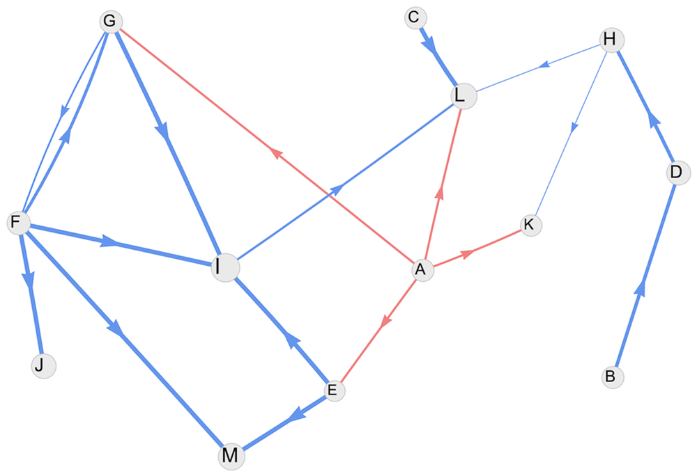
Figure 8. German FCM graph.
Table 4. German variables.
| node | value | rank | ent | ext | ord | id | od | deg | quart | variable description |
|---|
| A | 0.500 | 9 | 0 | 4 | 4 | 0.00 | 2.00 | 2.00 | Q1 | Natural Force Risks (Weather) |
| B | 0.500 | 9 | 0 | 1 | 1 | 0.00 | 0.80 | 0.80 | Q1 | Associations (Association,
Representation of interests,
Lobbying) |
| C | 0.500 | 9 | 0 | 1 | 1 | 0.00 | 1.00 | 1.00 | Q1 | Infrastructure |
| D | 0.599 | 6 | 1 | 1 | 2 | 0.80 | 0.80 | 1.60 | Q3 | Communication |
| E | 0.438 | 13 | 1 | 2 | 3 | 0.50 | 2.00 | 2.50 | Q1 | Soil |
| F | 0.555 | 7 | 1 | 4 | 5 | 0.41 | 3.70 | 4.11 | Q2 | Climate |
| G | 0.534 | 8 | 2 | 2 | 4 | 1.20 | 1.41 | 2.61 | Q2 | Biodiversity |
| H | 0.617 | 5 | 1 | 2 | 3 | 0.80 | 0.42 | 1.22 | Q3 | True Prices |
| I | 0.822 | 1 | 3 | 1 | 4 | 3.00 | 0.51 | 3.51 | Q4 | Ecosystem Services |
| J | 0.635 | 4 | 1 | 0 | 1 | 1.00 | 0.00 | 1.00 | Q3 | Climate Protection |
| K | 0.470 | 12 | 2 | 0 | 2 | 0.71 | 0.00 | 0.71 | Q1 | Production |
| L | 0.690 | 3 | 4 | 0 | 4 | 2.22 | 0.00 | 2.22 | Q4 | Income (Producers) |
| M | 0.730 | 2 | 2 | 0 | 2 | 2.00 | 0.00 | 2.00 | Q4 | Preservation for the Future |
The German graph is notably sparse (Figure 8), with only 18 connections among 13 variables. The variable A Natural Force Risks (Weather) occupies a central position within the German FCM network, acting as a key node that influences many other variables. its impact is notably negative, with this influence propagating throughout the grid. This central role highlights the importance of weather-related risks as a critical factors in the system, underscoring their pervasive effect on both environmental (i.e. physical) and economic (i.e. social) dynamics. The widespread propagation of this negative influence emphasises the challenges posed by natural forces, which can disrupt the stability and sustainability of the system as a whole. The importance of M Preservation for the Future emphasises Germany’s forward-looking orientation, reflecting a commitment to safeguarding agricultural and environmental systems for future generations. Together, German variables indicate a balance between addressing current economic needs, as represented by L Producers Income, and maintaining the long-term sustainability of both natural and human resources. This perspective aligns with Germany’s broader emphasis on integrating ecological stewardship with social and economic considerations.
The intensity of the links in the German FCM is relatively weak, with most connections contributing minimally to the overall dynamics of the system. This low intensity results and a mere density d = 0.12, the lowest observed in this study, indicates that the network is less interconnected compared to the other countries. Such sparse interconnections suggest a system where variables exert only limited influence on one another, leading to a more gradual propagation of changes through the network. This structural characteristic significantly contributes to a slower approach to equilibrium, as reflected in the convergence rate of k = 0.45, which is the slowest among all the countries analysed. The combination of weak links and low density implies that systemic adjustments and feedback mechanisms take more time to stabilise, potentially reflecting the cautious and deliberate nature of the system’s interactions. The German FCM stands out with the highest number of terminal nodes—a total of seven, including both drivers and receivers—compared to the other countries analysed. This highlights a system where a significant proportion of variables are either primarily influencing the network as drivers or being influenced as receivers, with limited intermediary roles. This structural characteristic suggests a network that is more linear in nature, with clear start and end points in its causal chains, reflecting a focused and streamlined representation of the system’s dynamics.
Italy
The Italian FCM (Figure 9) highlights three key variables in the fourth quartile: E Resistance and Resilience of the Productive System, K Farmers’ Quality of Life, and F Multifunctional Agriculture. Among these, K Farmers’ Quality of Life holds a particularly prominent position as a receiver variable, with no outgoing arrows. Importantly, it is conceptually distinct from Farmers’ Income in the original complete map, reflecting a broader perspective that includes well-being, work-life balance, and personal fulfilment, rather than purely economic measures [Foodlevers, 2023].
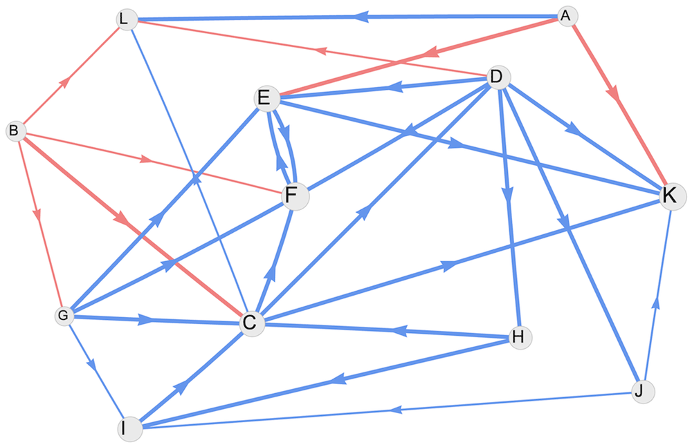
Figure 9. Italian FCM graph.
Additionally, E Resistance and Resilience of the Productive System emerges as a critical node of the FCM. This variable underscores the importance of ensuring that agricultural systems can withstand external shocks and adapt to changing conditions, reinforcing the sustainability and stability of the sector. Together with F Multifunctional Agriculture, these variables reflect a nuanced understanding of the interplay between social and physical issues, highlighting Italy’s commitment to balancing economic, social, and environmental priorities in its organic farming systems (Table 5).
Table 5. Italian variables.
| Node | value | rank | ent | ext | ord | id | od | deg | quart | variable description |
|---|
| A | 0.500 | 10 | 0 | 3 | 3 | 0.00 | 3.00 | 3.00 | Q1 | Climate Change |
| B | 0.500 | 10 | 0 | 4 | 4 | 0.00 | 2.50 | 2.50 | Q1 | Requirements for Premium
Resources |
| C | 0.798 | 4 | 4 | 4 | 8 | 4.00 | 3.50 | 7.50 | Q3 | Short Value Chain |
| D | 0.690 | 6 | 1 | 6 | 7 | 1.00 | 5.50 | 6.50 | Q3 | Collaborative Networking |
| E | 0.825 | 3 | 4 | 2 | 6 | 4.00 | 2.00 | 6.00 | Q4 | Resistance and Resilience of
the Productive System |
| F | 0.924 | 1 | 5 | 1 | 6 | 4.50 | 1.00 | 5.50 | Q4 | Multifunctional Agricolture |
| G | 0.438 | 12 | 1 | 4 | 5 | 0.50 | 3.50 | 4.00 | Q1 | Inner Areas Demography |
| H | 0.666 | 7 | 1 | 2 | 3 | 1.00 | 2.00 | 3.00 | Q2 | Ecological Biodiversity |
| I | 0.772 | 5 | 3 | 1 | 4 | 2.00 | 1.00 | 3.00 | Q3 | Food Local System |
| J | 0.666 | 8 | 1 | 2 | 3 | 1.00 | 1.00 | 2.00 | Q2 | Culture, Education, Awareness |
| K | 0.895 | 2 | 5 | 0 | 5 | 4.50 | 0.00 | 4.50 | Q4 | Farmers Quality of Life |
| L | 0.575 | 9 | 4 | 0 | 4 | 2.50 | 0.00 | 2.50 | Q2 | Hyrogeological Risks |
The driver A Climate Change acts as a significant external force, influencing multiple aspects of the agricultural sector, from productivity to sustainability. Similarly, B Requirements for Premium Resources highlights the dependency of the system on external inputs, perceived as critical for maintaining agricultural productivity. L Hydrogeological Risks, a receiver, reflects the system’s vulnerability to environmental challenges, such as floods and landslides, which are perceived as increasingly exacerbated by climate change.
The topology of the Italian FCM graph occupies a middle ground among all the case studies, with a density of 0.22, reflecting a moderately connected system. In terms of d, c, and h, the Italian map shows the greatest similarity to the Finnish one. However, it is important to note that the underlying agricultural systems of reference are fundamentally different. While Finland’s FCM emphasises social and cultural aspects, the Italian map incorporates a balanced perspective, capturing both resilience and human-centred outcomes, tailored to its unique agricultural and environmental context. This comparison shows how different contexts can give rise to relatively similar causal networks, reflecting shared structural features despite distinct thematic focuses and practical realities. The graph includes a single feedback loop, E-F, which has a limited impact on the overall system’s convergence rate. The convergence rate remains at an average value k = 0.69, indicating a steady approach to equilibrium.
The driver node B Requirements for Premium Resources, is particularly noteworthy for its exclusively negative arrows directed toward its prime-connected nodes. This pattern suggests a prevailing sense of skepticism or lack of trust toward the institutions or systems responsible for providing or managing subsidies. It highlights a perception that such requirements are more likely to impose constraints or challenges rather than supporting or fostering the agricultural system. This dynamic reflects deeper concerns within the stakeholder community about institutional reliability and the accessibility of high-quality inputs essential for sustainable agricultural practices.
Beyond topological affinity, it is worth highlighting the similarity between Italy’s K Farmers’ Quality of Life and Finland’s D Wellbeing of the producer (values), suggesting a strong connection to social values despite the geographical and cultural distance between the countries.
Poland
An important distinction emerges from the Foodlevers project: while most countries used Fuzzy Cognitive Mapping to explore the interplay among social, economic, and physical variables within their local systems, Poland took a markedly different approach. Instead of focusing on the relationships between variables, the Polish researchers utilised FCM to map the interactions and dynamics among the stakeholders themselves. This unique perspective shifts the focus from systemic factors to the actors driving the system, providing valuable insights into the social and institutional networks that underpin decision-making and influence system behaviour (Figure 10). Such an approach highlights the critical role of stakeholder relationships in shaping outcomes and offers a complementary lens for understanding and addressing complex systems. On the other hand, Polish results are not directly comparable with the other countries (Table 6).
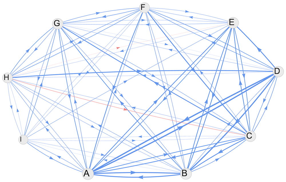
Figure 10. Polish FCM graph.
Table 6. Polish stakeholders.
| node | value | rank | ent | ext | ord | id | od | deg | quart | stakeholder description |
|---|
| A | 0.928 | 1 | 8 | 8 | 16 | 3.12 | 2.83 | 5.95 | Q4 | NGOs and educators |
| B | 0.911 | 2 | 8 | 8 | 16 | 2.77 | 2.10 | 4.87 | Q4 | Consumers |
| C | 0.822 | 6 | 8 | 8 | 16 | 2.15 | 2.36 | 4.51 | Q2 | Processors |
| D | 0.834 | 5 | 6 | 7 | 13 | 1.92 | 2.58 | 4.50 | Q2 | Media |
| E | 0.860 | 3 | 8 | 6 | 14 | 2.17 | 1.47 | 3.64 | Q3 | Detailers and
wholesalers |
| F | 0.768 | 7 | 8 | 8 | 16 | 1.44 | 2.17 | 3.61 | Q2 | Researchers |
| G | 0.845 | 4 | 8 | 8 | 16 | 2.09 | 1.44 | 3.53 | Q3 | Farmers |
| H | 0.735 | 8 | 8 | 8 | 16 | 1.22 | 1.60 | 2.82 | Q1 | Decision makers and
policy makers |
| I | 0.646 | 9 | 6 | 7 | 13 | 0.72 | 1.05 | 1.77 | Q1 | Suppliers |
A NGOs and educators, positioned in the fourth quartile, play a crucial role in shaping perceptions and fostering awareness of organic practices. Their influence highlights the importance of knowledge dissemination and advocacy in promoting sustainable food systems. Similarly, B Consumers, also in the fourth quartile, emerge as key drivers of demand, reflecting a growing societal awareness and preference for organic products. In contrast, E Detailers and wholesalers, situated in the third quartile, serve as essential intermediaries in the organic food chain, facilitating market access and distribution. Their position underscores the structural importance of supply chain actors, although their perceived influence remains slightly lower than that of A NGOs and Consumers. Finally, G Farmers, also in the third quartile, occupy a foundational role in the organic food system. Despite being central to production, their relatively lower placement suggests that challenges persist in empowering producers, such as limited resources or access to markets. The polish distribution of stakeholders’ values highlights the prominence of demand-side actors. H Decision makers and policy makers only fall in the first quartile.
The Polish FCM graph reveals a nearly saturated structure, showcasing a beautifully symmetrical organisation. All nodes are interconnected through pairwise feedback loops, reflecting a highly dynamic system. The strength of the causal connections exhibits considerable variability, ranging from 0.01 to 0.72, indicating the nuanced nature of stakeholder relationships within the organic food chain. Notably, the vast majority of these relationships are direct, with only 2 out of 68 connections being inverse. This highlights a system primarily driven by positive, reinforcing interactions, further contributing to the graph's cohesive and well-structured appearance, reflected by a k = 0.69 ensemble convergence rate.
Romania
In Romania, the FCM analysis reveals a distinct concentration of influence across key stakeholders (Figure 11). In the fourth quartile, K rural society, C education, I passion, and M organic producers stand out, showcasing a strong connection between local communities, knowledge dissemination, and intrinsic motivation in sustaining the organic food chain. These relationships highlight the social and emotional underpinnings critical for long-term success. In the third quartile, actors such as B politics, the F legal framework, and N farmer support appear, suggesting that governance and institutional structures are influential but not yet dominant forces (Table 7).
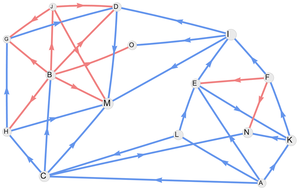
Figure 11. Romanian FCM graph.
Table 7. Romanian variables.
| node | value | rank | ent | ext | ord | id | od | deg | quart | variable description |
|---|
| A | 0.500 | 13 | 0 | 4 | 4 | 0.00 | 4.00 | 4.00 | Q1 | small producers |
| B | 0.680 | 6 | 1 | 6 | 7 | 1.00 | 6.00 | 7.00 | Q3 | Politics |
| C | 0.754 | 3 | 2 | 4 | 6 | 2.00 | 4.00 | 6.00 | Q4 | Education |
| D | 0.536 | 10 | 4 | 1 | 5 | 4.00 | 1.00 | 5.00 | Q2 | Investment |
| E | 0.609 | 9 | 3 | 2 | 5 | 3.00 | 2.00 | 5.00 | Q2 | Short food chain |
| F | 0.680 | 7 | 1 | 3 | 4 | 1.00 | 3.00 | 4.00 | Q3 | Legal Frame |
| G | 0.378 | 14 | 3 | 1 | 4 | 3.00 | 1.00 | 4.00 | Q1 | Market |
| H | 0.519 | 12 | 2 | 2 | 4 | 2.00 | 2.00 | 4.00 | Q1 | Consumer |
| I | 0.784 | 2 | 2 | 3 | 5 | 2.00 | 3.00 | 5.00 | Q4 | Pasion |
| J | 0.336 | 15 | 1 | 3 | 4 | 1.00 | 3.00 | 4.00 | Q1 | Bureaucracy |
| K | 0.752 | 4 | 2 | 2 | 4 | 2.00 | 2.00 | 4.00 | Q4 | Rural Society |
| L | 0.622 | 8 | 1 | 2 | 3 | 1.00 | 2.00 | 3.00 | Q2 | power of example |
| M | 0.829 | 1 | 6 | 0 | 6 | 6.00 | 0.00 | 6.00 | Q4 | organic producers |
| N | 0.696 | 5 | 3 | 0 | 3 | 3.00 | 0.00 | 3.00 | Q3 | farmer support |
| O | 0.526 | 11 | 2 | 0 | 2 | 2.00 | 0.00 | 2.00 | Q2 | Labor force |
The topology of the Romanian FCM graph reveals an interesting structural feature, with two nodes (C and I) acting as critical hinges that split the map into two interconnected subgraphs. These nodes serve as central bridges, ensuring connectivity between the otherwise distinct clusters of variables. The degree of these hinge nodes is notably high (deg C = 6, deg I = 5), highlighting their strategic position in the dynamics of the FCM. One of the subgraphs, located on the left side of Figure 11, features a notable concentration of inverse relationships, primarily centred around nodes B and J. This suggests that these nodes drive a contrasting dynamics within this section of the map, not influencing the right subgraph, since it is not causally connected to the left one: nodes C and I do not have any arrows originating from the left subgraph. All the connections strengths are ± 1, without intermediate values, like Finland’s FCM.
Notably, B Policy exerts exclusively very strong negative influences on the other variables within the system. A similar pattern can be observed in Italy, where policy-related variables also exhibit predominantly negative influences. This alignment may suggest a common trend of scarce trust in institutions, reflecting stakeholders' skepticism toward the role and effectiveness of local and European policy in supporting the organic food chain.
United Kingdom
A detailed analysis of the leverage points within the UK organic food chain has already been published [Staton et al., 2024b]. In this article, we focus exclusively on the main variables extracted from the full FCM (Figure 12). Despite the reduced number of variables, the resulting map remains notably complex, reflecting the intricate nature of the system even in its simplified form. The variables in the fourth quartile are well distributed across social, physical, and environmental domains. C Consumer willingness to pay for organic represents a key social and economic driver, emphasising the role of consumer behaviour in supporting organic markets. H Carbon sequestration, a physical-environmental variable, highlights the system’s contribution to climate mitigation and sustainability. Finally, M Evidence and awareness of biodiversity benefits underscores the importance of knowledge dissemination and ecological awareness in fostering stakeholder engagement. Together, these variables reflect a holistic perspective where economic incentives, environmental benefits, and societal awareness align to strengthen the organic food system's development and resilience (Table 8).
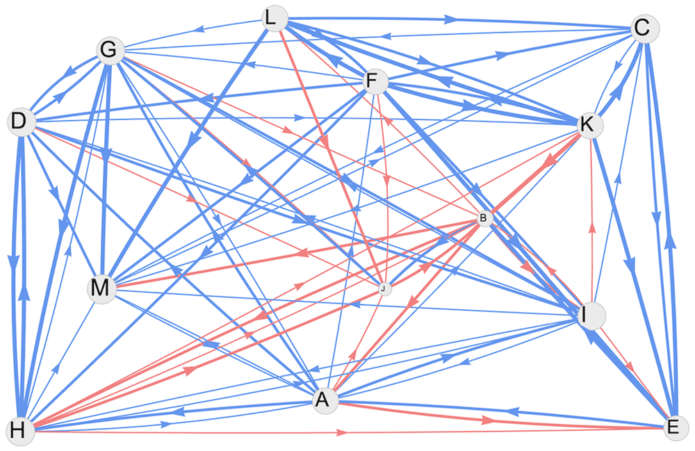
Figure 12. UK FCM graph.
Table 8. UK variables.
| node | value | rank | ent | ext | ord | id | od | deg | quart | variable description |
|---|
| A | 0.831 | 8 | 6 | 9 | 15 | 2.66 | 4.67 | 7.33 | Q2 | Landowner engagement with organic farming |
| B | 0.253 | 12 | 6 | 6 | 12 | 3.66 | 3.68 | 7.34 | Q1 | Short term thinking in economics |
| C | 0.965 | 2 | 6 | 4 | 10 | 4.00 | 1.66 | 5.66 | Q4 | Consumer willingness to pay for organic |
| D | 0.952 | 4 | 5 | 6 | 11 | 3.34 | 3.67 | 7.01 | Q3 | Soil health |
| E | 0.751 | 11 | 6 | 3 | 9 | 4.00 | 2.67 | 6.67 | Q1 | Food scares |
| F | 0.800 | 10 | 3 | 10 | 13 | 1.67 | 7.01 | 8.68 | Q1 | Farmer/ certification body relationships |
| G | 0.939 | 5 | 8 | 7 | 15 | 3.66 | 4.33 | 7.99 | Q3 | Carbon and biodiversity credits |
| H | 0.958 | 3 | 6 | 9 | 15 | 4.34 | 3.98 | 8.32 | Q4 | Carbon sequestration |
| I | 0.925 | 6 | 6 | 9 | 15 | 3.68 | 2.97 | 6.65 | Q3 | Water quality |
| J | 0.101 | 13 | 7 | 2 | 9 | 3.33 | 1.34 | 4.67 | Q1 | GHG emissions |
| K | 0.837 | 7 | 7 | 6 | 13 | 3.32 | 5.00 | 8.32 | Q2 | Fear of Genetically modified crops |
| L | 0.826 | 9 | 3 | 6 | 9 | 2.33 | 4.01 | 6.34 | Q2 | Transparency: consumer awareness of labels
and organic standards |
| M | 0.986 | 1 | 10 | 2 | 12 | 5.66 | 0.66 | 6.32 | Q4 | Evidence and awareness of biodiversity
benefits |
Remarkably, two variables exhibit particularly low values: J GHG emissions (0.10) and B Short-term thinking in economics (0.25). While these values appear minimal, their semantic content reveals that they represent negative outcomes. Therefore, from the perspective of fostering organic farming, it is actually encouraging that these variables hold such low significance, as it suggests reduced environmental harm and a focus on long-lasting economic priorities.
The UK FCM is notably complex, featuring a significant number of causal connections across 13 variables. This results in a graph density of 0.51, the second highest after Poland and considerably higher than those of all other countries analysed. The connection strengths in the UK FCM have been derived from the original data collection, where stakeholders indicated relationships as low, medium, or strong, assigning values of ±0.3, ±0.5, and ±0.7 [Staton et al., 2024b]. These qualitative inputs have been rescaled to the numeric values ±0.33, ±0.67, and ±1 [Foodlevers, 2023].
The number of inverse relationships in the UK FCM is consistent, reflecting a thorough and nuanced analysis of the organic food system variables and their complex interdependencies [Staton et al., 2024b]. The German FCM graph (Figure 8), also based on 13 variables, clearly shows the difference of density (German d = 0.12 versus UK d = 0.51).
The UK FCM exhibits the highest hierarchy among all analysed countries, with a value of h = 0.49, which is twice the mid-range values observed in our comparative analysis for Finland and Italy. This indicates a more structured and directional system, where certain nodes exert a clear influence over others, leading to a pronounced top-down flow of causal relationships. This structural feature is also reflected in the highest ensemble convergence rate, with a value of k = 0.77. Many short feedback loops can be spotted in the graph.
Discussion
A note about ensemble dynamics
Our FCMs were developed through dedicated workshops conducted with stakeholders, employing a variety of techniques for data collection to ensure comprehensive input. The raw data were subsequently summarised and homogenised to maintain consistency and comparability across different datasets. These standardised datasets were then analysed in the R environment using the tools provided by the fcm package, which facilitated the processing, analysis, and interpretation of the FCMs through its diverse set of functions tailored for FCM modeling [Dikopoulou & Papageorgiou, 2022; Papageorgiou, 2011; Papageorgiou, 2014; Stylios & Groumpos, 1999].
The R fcm package provides several methods for analysing and interpreting FCMs, each based on a specific inference rule. These include Kosko K, Equation (2a), Modified Kosko MK, Equation (2b), Kosko-clamped KC, and Modified Kosko-clamped MKC. The K method follows the classic Kosko inference rule [Kosko, 1986], which calculates the value of concepts based on initial values and the weight matrix. The MK method is a modified version of Kosko's rule, incorporating adjustments such as weighted influences. The KC method applies the Kosko rule in a clamped manner, which stabilises the output over iterations, while MKC builds on this by clamping the modified Kosko approach. In our study, we primarily focused on the K inference rule, but we also tested the MK, KC, and MKC methods. While these alternative methods provided different final numerical values, they consistently produced nearly the same rank of variables, confirming the robustness of the rankings across inference rules. Figure 13 shown an example of difference of ranking between K and MK inferences for United Kingdom. The MK values have a median shift of +0.07 with respect to the corresponding K values. The only differences in rank are between variables A and L.
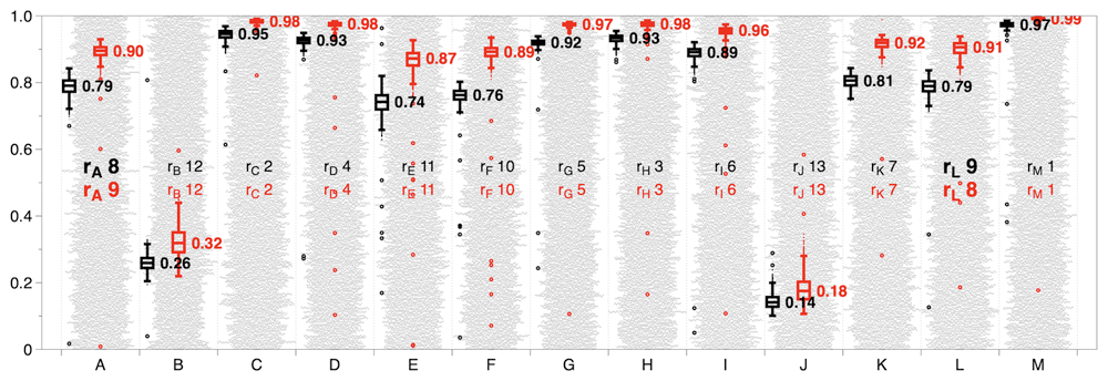
Figure 13. United Kingdom Kosko (black) vs Modified Kosko (red) ensemles.
Figure 13 illustrates the distribution of initial conditions for each variable, visualised as a grey cloud representing the spread of random initial values. Superimposed on this are box plots, which show the distribution of each variable at the 3rd iteration, including outliers. Variables A and L ranks are highlighted in bold: rA = 8 (K) and 9 (MK), while rL = 9 (K) and 8 (MK), their differences are negligible: |VA - VL| = 0.0106 (K) 0.0012 and (MK) . The same pattern is observed in the results for the other countries, with even less variability in the distribution of variables across iterations, thus reinforcing the robustness of the variables ranking, given an assumed ergodicity of the system [Durlauf, 1999; Peters, 2019; Tsallis et al., 2003].
The rescaled and rescaled clamped methods, also available in the fcm package, operate by expanding the variable values to cover the entire [0,1] range during each iteration of the algorithm. In fact, after each application of Equation (2), this rescaling ensures that concept activation levels remain within normalised bounds, potentially enhancing interpretability and compatibility with specific modeling scenarios. However, when applied to our FCMs using a random initial conditions ensemble approach, we did not achieve convergence [Garlaschelli & Loffredo, 2014]. This lack of convergence suggests that the dynamic rescaling process, particularly in maps with complex interconnections or feedback loops, may introduce oscillations or instability that prevent the system from stabilising to a fixed point in the variables space (a n-dimensional unitary cube).
Conclusions
The application of statistical physics techniques, particularly the concept of ensemble averages [Sethna, 2021], enabled us to identify stable values for all the variables included in the examined FCMs. Through the ensemble average approach, we aggregated the results over a range of initial conditions, smoothing out variability and ensuring robust estimates of the variables' steady-state behaviour. This methodology proved effective in stabilising the system and provided reliable insights into the dynamics and interactions of the FCM components [Castellano et al., 2009; Contucci & Vernia, 2020]. Stemming from ensemble dynamics, the semantic analysis of FCMs variables revealed unique leverage points and structural dynamics for each country, reflecting diverse stakeholder perceptions of the organic food chain.
In Belgium, key variables such as consumer demand, sector size, societal awareness, and the number of innovative organic farms highlight the focus on market dynamics and public engagement. Feedback loops and driver variables emphasise rapid system responses, though the absence of physical measures points to an under-explored area in sustainability assessment.
In Germany, sustainability and economic viability are central, with variables such as ecosystem services, producers' income, and preservation for the future shaping the system. Sparse interconnections and low-density networks indicate a cautious, gradual approach to equilibrium, with natural force risks playing a significant negative role. Germany's FCM reflects a balance between current needs and future-oriented ecological stewardship.
For Finland, the FCM emphasises social and cultural dimensions, with variables like public awareness, media discourse, and producer well-being shaping the organic sector. Simplified weights of ±1 reflect a clear directional influence but lack intensity differentiation. Media narratives and human connections emerge as critical drivers for Finland’s organic food system.
Italy emphasises resilience and human-centred outcomes, with key variables including farmers' quality of life, resistance to shocks, and multifunctional agriculture. The system’s moderate density balances economic, social, and environmental priorities. However, skepticism toward institutional support underscores concerns about resource dependencies and policy effectiveness.
In Romania, rural society, education, and organic producers play pivotal roles. Skepticism toward policies mirrors concerns in Italy, while a bifurcated graph structure highlights contrasting dynamics between connected subgraphs.
The United Kingdom demonstrates a holistic system, integrating social, physical, and environmental factors. Variables like consumer willingness to pay, carbon sequestration, and biodiversity awareness underscore a balanced approach to sustainability. High graph density and strong hierarchical structure suggest a complex, directional system with rapid convergence to equilibrium.
Finally, in Poland the FCM shifts focus to stakeholder dynamics, revealing the importance of NGOs, educators, and consumers in driving awareness and demand. High graph density and interconnected relationships reflect a dynamic and collaborative network, but challenges persist in empowering producers and addressing institutional trust.
Our findings demonstrate how comparable structural features in FCMs can manifest in distinct ways, shaped by the unique dynamics of local contexts and the diverse perceptions of stakeholders, highlighting the adaptability and versatility of Fuzzy Cognitive Mapping as a methodological tool. By integrating methods from statistical mechanics, we have enhanced the robustness and analytical depth of Fuzzy Cognitive Mapping, maintaining a consistent analytical framework and providing a nuanced understanding of the intricate interconnections within diverse systems dynamics.