Introduction
The optimization of building energy operations using analytic tools like automated fault detection and diagnosis (FDD) has the potential to generate significant energy savings and to contribute to global efforts to reduce greenhouse gas emissions. Several pilot projects worldwide have demonstrated average energy savings of about 10% through the implementation of FDD (Kramer et al., 2020). Currently, most commercially available FDD solutions rely on rule-based systems, which are valued for their simplicity and high specificity (low false-positive alarm rate). However, these systems require numerous parameters and considerable effort for setup, tuning, and maintenance, which can impede their transferability from one system to another. Moreover, it is essential to minimize the implementation costs of FDD to ensure a swift return on investment (Lin et al., 2020).
Recently, Mirnaghi and Haghighat (2020), Melgaard et al. (2022), and Matetić et al. (2023) have focused on the application of machine learning (ML) methods in the FDD process. They showed that they could reduce the modelling efforts and improve the model transferability by learning the dynamic behaviour of systems from historical operating data. If well-trained, ML models can perform as effectively as rule-based systems and even detect novel fault patterns for which no predefined rules exist. However, despite extensive research, ML-based FDD solutions are rarely implemented in practice for the supervision of Heating, Ventilation, and Air Conditioning (HVAC) systems. This is largely due to challenges in the need for high-quality training data as well as the requirement for specialized expert knowledge for applying and interpreting ML results effectively. In particular, one of the biggest barrier for applying ML-Models in buildings is the lack of labelled faulty operation data of the targeted systems, which significantly hamper training the models on faulty behaviours. An approach to address this problem is a residual generating FDD process, as shown in Figure 1, inspired by Ding (2013). Here, the nominal behaviour is modelled and the differences between the estimates and the observed data are calculated. In the event of a fault, the generated residuals carry information about the abnormal behaviour of the system. By evaluating the patterns in the residual vector, a decision can be made about the overall fault status (detection) and gather further information about the observed fault type (diagnosis).
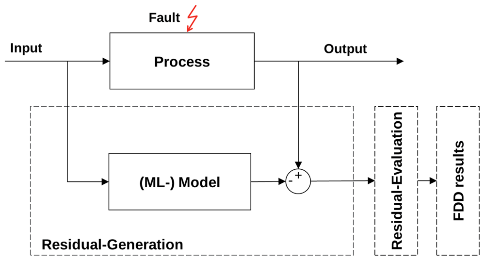
Figure 1. Scheme of a residual generating FDD process.
To reduce the implementation efforts and enhance the transferability of the ML-models, we propose a methodology that integrates two distinct AI methods to model a highly automated residual-generating FDD approach. By filtering historical operating data through a rule-based system developed in (Rist et al., 2022), the objective is to ensure that the data used for training the ML models is mostly fault-free, thus eliminating the need for time-consuming manual checks. In the application phase, both systems operate in parallel, which enables the use of a reduced set of rules with fewer parameters, with the objective to enhance the quality of the FDD results. Furthermore, we aim to enable a better interpretation of the ML models through integrating them into the residual-generating approach and thereby to improve transparency in the decision-making process. To assess performance and transferability, we applied our method to nine air handling units (AHUs) across three different buildings. Although this work focuses on AHUs, the method can also be extended to other components of HVAC systems in buildings.
Methods
The integration of expert rules and ML models into a residual-generating FDD approach is illustrated in Figure 2. Initially, time-series data from the Building Automation System (BAS) is analysed using an extensive set of "if-then" rules specifically designed to detect faults in HVAC systems. It also incorporates the automated discovery of data points and plant topologies, based on unified semantics, ensuring adaptability to various system configurations and setups. Based on the available data points (sensors, actuators, operation signals), these rules are automatically triggered, and each rule generates a binary signal (0: fault-free, 1: faulty) when the data points used as inputs in the rule are available. This first step enables the detection of known and frequently occurring faults. The results from the rule-based system are then used to filter the time-series data used to train the ML models for residual generation. Based on the training results, the parameters for the subsequent residual scoring (evaluation) and fault detection are determined automatically. In the application phase, data from the Building Automation System (BAS) is analysed by both methods in parallel, and a final fault signal is triggered if one of the methods detects a faulty state.
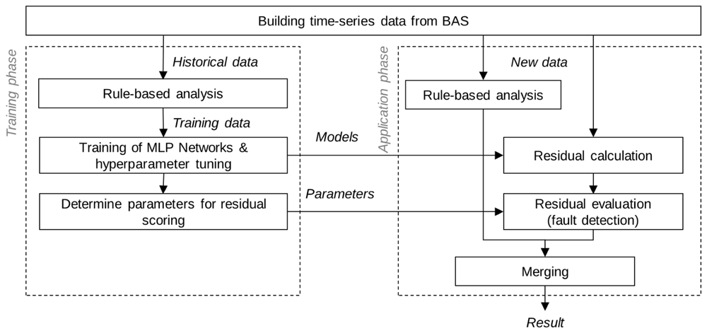
Figure 2. Scheme of the proposed methodology to model a fully automated residual generating FDD approach for HVAC systems.
For residual generation, we apply a bank of Multilayer Perceptron (MLP) models, with hyperparameters tuned through Bayesian optimisation. For each observed data point, a separate regression model for continuous variables or classification model for discrete variables is trained. The nominal behaviour of the targeted system is thus described through a set of ML-models. The input data for each ML-model are all recorded data points, except for the estimated variable itself. For example, in the analysed case studies, models with 10–20 input variables like e.g. outdoor and return air temperatures, valve and pump signals, etc. were employed to estimate the supply air temperature. To capture the system's dynamic behaviour, a sliding time window of two hours is applied. Table 1 presents the selected hyperparameters of the MLP models. Further details regarding the performance of this modelling approach can be found in Dietz et al. (2023), whereby the same case studies and time periods of the data sets are considered in this study. It is important to note that any type of ML model can be used if it estimates the nominal behaviour of the system with sufficient accuracy. The estimation and subsequent calculation of the residuals to the observed data are performed at discrete time intervals, determined by the logging frequency of the BAS. Periods with incomplete data records are excluded from the analysis.
Table 1. Hyperparameters of the Multilayer-Perceptron models.
Range based values are selected by applying Bayesian optimisation.
| Hyperparameter | Value |
|---|
| Maximum number of epochs | 35 |
| Batch-size | 288 |
| Learning rate | 1e-4, 1e-5 |
| Loss function regression | Root mean squared error |
| Loss function classification | Cross-entropy |
| Number of hidden layers | 3–6, step 1 |
| Number of neurons in each layer | 24–552, step 48 |
| Dropout first hidden layer | 0,1 |
| Dropout 2nd to n hidden layer | 0,2 |
| Activation function | ReLu |
| Scaling method | Min-max scaling |
| Encoder (classification) | One-hot encoder |
Normalising the estimates to a range from 0 to 1 results in residuals ranging between -1 and 1, whereby a value of zero indicates the absence of faults. However, when a fault occurs, the validity range of the models may be exceeded, causing the estimates to fall outside the normalised range. In these cases, the estimates lose their physical significance, prompting us to constrain the residuals. Consequently, the residual vector for further evaluation is formulated as follows:
Where : residual vector; : observations and : estimations at time t.
A major challenge in residual evaluation is distinguishing between model uncertainties and fault effects. Uncertainties are significantly influenced by the chosen ML model and its ability to represent the dynamic behaviour of the system. A preliminary careful model selection is essential. However, the accuracy of estimation is heavily affected by the distribution of historical data and the range of represented operating conditions. Moreover, HVAC systems may switch between different operating modes (e.g., heating or cooling) accordingly to their control rules. Consequently, certain operating modes may be underrepresented in the data and, therefore, insufficiently learned by the model.
It is important to acknowledge that individual residuals result in different sensitivities of the FDD method at various value ranges, which depend on the related variable (such as control signal or temperature) and the particular type of fault. Even if the units are identical or normalised to a uniform value range (0–1), individual variables may still respond more strongly to faults. This presents a significant challenge, as the residual magnitude cannot be directly used to assess the impact of a fault. A particular difficulty arises with discrete variables, such as on/off signals that have only 0 or 1 values. An incorrect estimate immediately leads to high residuals, which can result in a high rate of false-positive alarms about the system's fault state.
To evaluate residuals and achieve reliable fault detection, we apply a variable tolerance band and scoring method as proposed by Dietz et al. (2024). The scoring of residuals aims to normalise the sensitivity range of the FDD method for each residual, thereby enabling an equal assessment. The parameters used to define the scoring functions are derived from the percentiles of the fault-free residual distribution during the training and validation period. To establish a scoring grid, ten percentile ranks, equally distributed around the median (see Table 2), are selected. Here, p1 sets the tolerance band around the median (Scoring = 0), while p5 defines the upper bound from which the maximum score value is assigned (Scoring = 1). Intermediate scores are linearly interpolated between the percentiles. Figure 3 illustrates the resulting scores (red line), underlaid with a histogram of supply air temperature residuals for both faulty (red) and fault-free (blue) data. The grey dashed lines indicate the percentiles used for linearised scoring.
Table 2. Rank of percentiles and their associated scoring values for residual evaluation.
| Percentile | Percentile Rank | Scoring Value |
|---|
| p1,low / p1,high
| 1.50% / 98.5% | 0.00 |
| p2,low / p2,high
| 0.50% / 99.5% | 0.25 |
| p3,low / p3,high
| 0.20% / 99.8% | 0.50 |
| p4,low / p4,high
| 0.10% / 99.9% | 0.75 |
| p5,low / p5,high
| 0.05% / 99.95 | 1.00 |
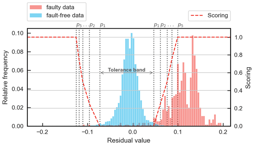
Figure 3. Histogram of supply air temperature residuals (MSA, AUD-8) for faulty (red) and fault free data (blue).
The grey dashed lines show the percentiles used for linearised scoring.
The procedure is repeated for each operating mode of the air handling unit (AHU) to establish a dynamic tolerance band over time. For this purpose, the current mode is determined through a set of rules that are automatically triggered based on available data points. The rule set identifies six distinct operating modes corresponding to the air conditioning functions of the analysed AHUs: fresh air, fresh air with activated heat recovery bypass, heating, heating with return air fraction, cooling, and cooling with return air fraction. No evaluation is performed when the AHU is off.
The total score is then calculated to assess the overall health status of the system. If the total score exceeds a predefined threshold level (Jth,s), a fault signal (FS) is activated (Formula (2)). This threshold allows adjusting the FD sensitivity during the application phase, and we set it at 1.5 across all case studies. However, the method can generate false positives during the transition between operational modes. Therefore, in this study a fault detection alarm (FDt) is only triggered if the fault signal remains true for more than two consecutive time steps (Formula (3)). It may be necessary to increase the number of consecutive timesteps for shorter log intervals to ensure that transient states are accurately filtered out.
Where FDt : fault detection alarm; FSt : fault signal; si,t : score for residual i; Jth,s : threshold.
Description of the case studies
We evaluated the proposed methodology using data from nine AHUs located in three separate European buildings. The operational data was obtained from a BAS and no additional sensors have been installed. The datasets included status and flow variables such as temperature, pressure, humidity, and volume flows, along with control signals for actuators like valves, fans, and dampers. Energy or power data was not available for all AHUs and was therefore excluded from the fault detection (FD) process. Depending on the AHU being observed, this resulted in the creation of 11 to 22 ML-models whose residuals could be evaluated.
Case study MSA
The Maison du Savoir (MSA) building, which houses the lecture halls and rectorate of the University of Luxembourg, includes three AHUs with identical topologies from which data is used in this study. Each AHU is designed to supply fresh air, heating, and cooling to a specific auditorium. The units are equipped with a heating coil, an adiabatic cooling system, a heat recovery wheel, filters, and dampers that allow for operation in return air mode. In adiabatic cooling mode, water droplets are sprayed into the extracted air stream and subsequently evaporated causing a reduction of its temperature. Through the rotation of the heat recovery wheel, the supply air stream is also cooled down.
The AHUs differ in nominal volume flow rates (AUD2: 5250 m3/h; AUD7: 8,400 m3/h; AUD8: 3,150 m3/h). Volume flow is controlled in two stages (60%/100%) based on the zone's actual needs. Data acquisition began in May 2021, with measurements taken at five-minute intervals. Due to a significant modification in the control strategy—specifically the introduction of variable air flow based on CO2 measurements—only data collected up to mid-October 2022 is considered. The data is divided as follows:
Training period: 2021-05-19 to 2022-01-18
Validation period: 2022-01-19 to 2022-07-18
Test period: 2022-07-19 to 2022-10-18
Case study GSHN
The second case study is a primary school in Hohen Neuendorf (PSHN), Germany. Two AHUs, ZONE-A (3,150 m3/h) and ZONE-B (2,850 m3/h), supply ventilation to areas consisting of eight and six classrooms, respectively. A third AHU, SPO-HALL (3780 m3/h), serves the sports hall, including its changing rooms and showers. The building uses a hybrid ventilation system, incorporating both mechanical ventilation and natural ventilation through motorised openings. The AHUs operate in two stages, with the second stage activated during extreme hot or cold weather conditions when natural ventilation openings remain closed.
Each AHU is equipped with a heating coil, a plate heat exchanger for heat recovery, outside air dampers, and filters. Additionally, radiators within the zones control the room air temperature. We utilized data collected at five-minute intervals during the following periods:
Training period: 2015-01-01 to 2015-12-31
Validation period: 2016-01-01 to 2016-12-31
Test period: 2017-01-01 to 2017-12-31
Case study ISC
The third case study focuses on a boarding school facility in Luxembourg. One of the AHUs (LAB, 3000 m3/h) supplies laboratories area and is equipped with a plate heat exchanger, supply and extract air fans with pressure-controlled air flow, filters, and a heating coil. The second system (THEA) serves a theatre room with a CO₂-controlled volume flow (6,000 m3/h). The supply air is heated by a heating coil, and heat recovery is facilitated by a recovery wheel. Additionally, a residential building is ventilated by the third system (RESI), which includes a heat recovery wheel and heating coil. This system maintains a minimum volume flow of 2,200 m3/h, which increases based on humidity levels in the sanitary rooms, reaching a maximum of 5,000 m3/h.
Data collection was not uniform across all points, with some being event-based, which introduced challenges in preprocessing. However, for fault detection and diagnosis (FDD), the data was aggregated at 10-minute intervals. The periods for model training and FDD performance analysis are as follows:
Training period: 2017-01-01 to 2017-12-31
Validation period: 2018-01-01 to 2018-12-31
Test period: 2019-01-01 to 2019-12-31
These case studies, and their corresponding data sets, capture a wide range of system types, boundary conditions, available data points, time resolutions, and dynamic behaviours, reflecting conditions commonly encountered in practical applications. Each data set was manually analysed and labelled regarding the fault status and type.
Results
The proposed methodology for an automated FDD process was applied to each AHU without adjusting the parameters of residual generation, to assess its level of automation and the performance of fault detection when transferred to new systems. This approach also enables a comparison of the results from each use case. Only the thresholds for the rule-based system were adjusted to match the specific configurations of each system. Table 3 shows the number of automatically triggered rule sets (nrules).
During training, our methodology's rule-based analysis filters faulty operating states from the historical dataset. Without this filtering, the model might learn faulty behaviours, leading to predictions of faults as normal operations. This weakens the residuals, risking missed alarms and creating a seemingly effective model that could finally prove unreliable for fault detection and diagnosis. To assess the impact of faulty operating states on model performance, training was conducted both with and without prior filtering of faulty states.
Table 3. Summary of fault rates in the training and test datasets, number of considered rules (nrules), fault detection rates (FDR) for individual methods and the hybrid approach, and false alarm rates (FAR) caused by the residual-generating method.
| System | Fault rates | Rule-based
system | Res.-gen.-method
(without filtering) | Hybrid Approach |
|---|
| | Training in % | Testing in % | nrules | FDR in % | FAR in % | FDR in % | FAR in % | FDR in % |
|---|
| PSHN | ZONE-A | 10.7 | 1.7 | 6 | 14.5 | 0.5 | 26.7 | 0.5 | 40.3 |
| ZONE-B | 4.8 | 4.0 | 6 | 5.8 | 1.3 | 54.3 | 1.9 | 66.1 |
| SPO-Hall | 2.4 | 0.5 | 6 | 36.1 | 0.4 | 3.4 | 0.4 | 58.8 |
| MSA | AUD2 | 40.9 | 90.7 | 12 | 65.8 | 45.0 | 85.9 | 34.2 | 83.6 |
| AUD7 | 5.3% | 20.6 | 12 | 6.3 | 3.2 | 1.7 | 2.6 | 77.1 |
| AUD8 | 6.2 | 5.6 | 12 | 13.7 | 1.2 | 82.1 | 3.7 | 97.0 |
| ISC | THEA | 0.5 | 0.1 | 9 | 0.0 | 0.2 | 0.0 | 0.1 | 25.0 |
| LAB | 0.5 | 0.1 | 9 | 13.5 | 0.2 | 12.2 | 0.4 | 31.8 |
| RESI | 0.2 | 0.5 | 11 | 61.0 | 1.0 | 79.2 | 1.0 | 84.4 |
Figure 4 (left diagram) shows the change in the mean of the normalised mean absolute error (nMAE) for estimating nominal (fault-free) behaviour due to filtering. The nMAE represents the model's accuracy in predicting the nominal behaviour, where a lower nMAE indicates better alignment between the model's estimates and the actual values. The change in nMAE helps evaluate how effectively filtering faulty states impacts the quality of the model's estimates. For most of the investigated case studies, filtering out faulty states in the training data resulted in minimal changes to the mean, with deviations of less than ±0.5%.
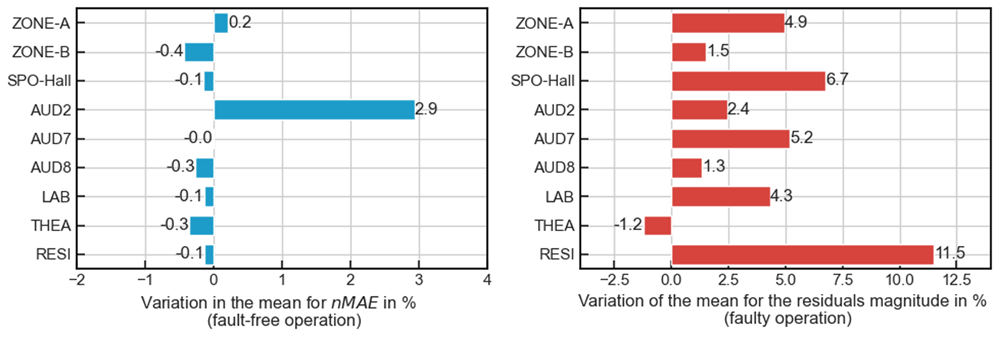
Figure 4. Left. Variation in the mean normalised absolute error (nMAE) for the estimate of fault free operation in the test period resulting from filtering faulty operating states in the training dataset. Right. Variation in the mean residual magnitude for faulty operating states across the evaluated case studies.
An exception is noted for AHU AUD2 in the MSA building, which shows a high proportion of faulty operating states in the training data (41%, Table 3) due to a valve leakage in the heating coil's hydraulic circuit. This indicates that filtering can reduce the model's generalisation ability, thereby adversely impacting the estimation of nominal behaviour. Conversely, stricter filtering of the training data confines the model's validity range to nominal behaviour during the training period, which benefits FDD by generating higher residuals in the presence of faults.
Figure 5 exemplary shows the impact on residuals during faulty operating states for both a continuous variable (supply air temperature after heat recovery) and a discrete variable (control signal of the return air damper) of the AHU AUD7. Filtering the data shifts the relative frequency of residuals to a higher value range and enhance the sensitivity of the method. A broader analysis, as depicted in the right diagram of Figure 4, shows that filtering raises the mean value of residual magnitude across all variables in nearly all case studies. It is important to note that the mean value also includes variables that might not be affected by any of the existing types of faults, so individual variables may be significantly more affected. Furthermore, the fault ratios, types of faults, and fault size significantly influence the extent of this shift. Due to the small fault ratios of less than 0.5% in the data (see Table 3), the results for the ISC building (LAB, THEA, RESI) are subject to a high degree of uncertainty. For example, the failure to detect a single fault can lead to a notable decrease in the FDR, as can be seen from the THEA case study. Nonetheless, the analysis reveals an overall increase in sensitivity.
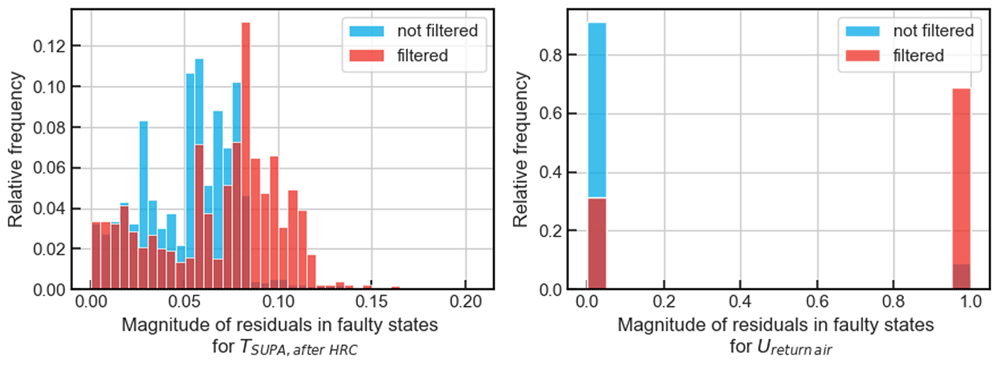
Figure 5. Relative frequency in the event of a fault for the residuals magnitude of supply air temperature after heat recovery (TSUPA,after HRC) and the control signal of the return air dampers (Ureturn air) of AHU AUD7 in the MSA building (test period).
The results are shown without filtering of the faulty operating states for model training (blue) and with filtering (red).
Prior filtering is also necessary for the automated parameterisation of the implemented residual evaluation procedure, as the support values for linear scoring—represented by percentiles—are determined based on the frequency distribution of residuals during the training period. Although this approach is robust to single faults, frequently occurring faults can shift the percentiles towards larger residual values. This results in a higher tolerance and thus to a reduced sensitivity in fault detection.
Figure 6 illustrates the evaluation procedure based on time series of three selected residuals from AHU AUD8 in the MSA building over a one-day period (left), depicting a summertime scenario with adiabatic cooling mode. For dynamic scoring, the dotted black line and the red line represent the lower (p1) and upper (p5) boundaries, respectively, derived from the percentiles. The figure also shows the individual scores (middle) and their sum of all evaluated variables, as well as the outcome of the fault detection (FD) logic (right). During the cooling system refill process, the cooling function is temporarily disabled, causing the bounds for scoring to vary in steps based on the current operating mode. The labelled fault (FStrue) indicates an unsuccessful attempt to refill the system due to an interrupted water supply, preventing cooling for the supply air. This fault was identified through a manual labelling process as the rule-based system did not include a rule to detect this kind of faults. This step in the labelling process highlights the drawbacks of rule-based FDD, which might be incomplete and require an expert to adapt them to new system configurations.
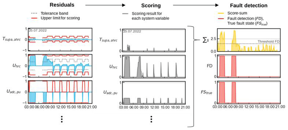
Figure 6. Illustration of the residual evaluation procedure based on time series.
Left. Time series of three exemplary residuals with the lower (p1, black dotted line) and upper (p5, red line) bounds used for dynamic scoring. The depicted variables include the supply air temperature after heat recovery (Tsupa,ahrc), the control signal of heat recovery (Uhrc), and the control signal of the adiabatic cooling pump (Uadc,pu). Middle. Individual residual scoring results. Right. Sum of all evaluated residuals, the outcome of the fault detection (FD) procedure, and the true fault state (FStrue).
The observed faulty behaviour causes high residual values, especially for the control signal of the heat recovery wheel (Uadc,pu) and the circulation pump of the adiabatic cooling system (Uhrc). In contrast, the residuals of the supply air temperature after heat recovery (Tsupa,ahrc) are nearly unaffected. As a result, the overall score (∑s) increases, and the fault can be correctly detected. The cooling system then operates without any issues for the rest of the day. During the filling process, the temperature changes cause the heat recovery to temporarily switch off before gradually ramping up to full capacity. These dynamics result in occasional spikes in residuals and, subsequently, in the calculated total score at regular intervals. However, the duration filter prevents any alarms from being triggered.
This example also demonstrates that the partial results of the residual-generating approach provide valuable information for manually analysing the source of specific faults as part of continuous commissioning. The high residuals for the heat recovery control signal indicate a lack of heat transfer in the supply air stream. Similarly, the pump signal residuals point to a malfunction in the adiabatic cooling system during the detected period.
Figure 7 shows boxplots of the resulting fault detection rates (FDR) and false alarm rates (FAR) during the test period, representing the application scenario for the rule-based system (blue), the residual-generating approach without prior filtering of the training data (grey) and for the hybrid approach, combining both methods (red). For comparison, the fault detection (FD) and actual fault state (FStrue) signals are processed identically, including the filtering of short-term positive values according to Formula (3). Moreover, the evaluation is conducted only when the system is switched on. However, unlike the residual-generating approach, rule-based detection can also be applied when the system is off, e.g., to detect an incorrect damper position.
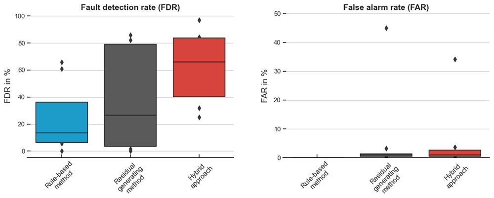
Figure 7. Boxplots illustrating the fault detection rates and false alarm rates for the residual-generating method without filtering (grey), the rule-based system (blue), and the hybrid approach during the test period.
Each box represents data from five of the nine case studies, with the line within the box indicating the median.
The residual-generating approach outperforms in identifying unknown faults, whereas rule-based fault detection (FD) is limited to faults whose symptoms are captured by predefined rules. Furthermore, it is often infeasible to define rules for every type of fault due to the limited number of available data points. In contrast, the residual-generating approach learns the system's dynamic behaviour, enabling the detection of faults that might not be directly observable in individual variables. These characteristic differences are evident in the results: the residual-generating approach demonstrates a higher sensitivity, resulting in improved FDR in most of the observed AHU systems. The rule-based system achieves a median FDR of 14%, while the residual-generating method reaches 27% and the hybrid approach significantly enhances the FD performance, achieving a median FDR of 66% and a lower spread of the results.
Examining individual results as shown in Table 3 reveals some challenges. For instance, during the test period for AHU THEA, both the rule-based method and the residual-generating approach show an FDR of zero. This highlights a difficulty in performance evaluation of real HVAC systems, as the low fault occurrence for this system resulted in a substantial reduction in the FDR.
The residual-generating approach, however, is prone to generating more false alarms (FAR: false alarm rate) than the rule-based system, which has generally a very low FAR if it is well parametrised, and only appropriate rules are applied for the given system configuration. FARs are particularly likely in ML FDD when the nominal behaviour cannot be sufficiently learned from training data or when the boundary conditions change during the application phase. In the case studies, AHU AUD2 exhibits a high FAR of 45% if the training data is not filtered, primarily due to constant leakage in the heating coil valve during the training phase, which prevents adequate learning of nominal behaviour. In general, low FARs were observed for the other AHUs, with the lowest rates (<1%) occurring in systems with a small number of fault states. By filtering the faulty states during training in the hybrid approach, the percentiles of the residuals for scoring fit better to the nominal behaviour, reducing the tolerance band and enhancing sensitivity without increasing false alarms. The median FAR remains at 1%, with only minor variations observed across individual systems.
Time series examples are given in Figure 8. The left diagram illustrates a case where the residual-generating approach demonstrates higher sensitivity to detect faults. The data shows a valve leakage in AHU ZONE-B. Although the heating control valve appears to be closed, a constant volume flow can be observed in the hydraulic circuit. Consequently, heat is continuously supplied to the supply air stream, causing the system to open the bypass of the heat recovery unit, despite low outside air temperatures below 5°C, in order to maintain the setpoint values for the supply air temperature.
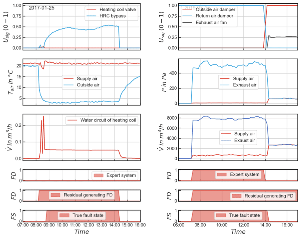
Figure 8. Exemplary time series illustrating observed operating faults and the corresponding results of each fault detection method.
The diagram on the left shows a leakage in the heating coil valve (ZONE-B), while the diagram on the right depicts overpressure in the exhaust air duct (RESI).
In this case study, analysing the temperature difference across the heating coil is not possible because the necessary temperature measurements are not available. As a result, manual or control-based detection of this fault type can only be done if the volume flow in the hydraulic circuit is considered. However, the volume flow in the hydraulic circuit is not part of the standard set of installed sensors and was only recorded separately as part of a research project. Therefore, the automated fault detection (FD) is carried out without considering the volume flow. This example illustrates a significant advantage of the residual-generating approach: by modelling the system behaviour, many different types of faults can be detected even with a small number of available data points.
Another example, where the fault is detected by both systems, is shown on the right side of Figure 8. Although the operating signal indicates that the extract air fan is switched off and the fresh air dampers are closed, there is a clear overpressure in the extract air duct. However, because the residual-generating approach analyses a sliding time window, an error signal is generated that lasts longer than the actual fault period, leading to false alarms.
Conclusion
In this paper, we propose a methodology that combines two distinct AI methods to create a highly automated residual-generating fault detection and diagnosis (FDD) process. This approach aims to reduce implementation efforts by minimizing manual configuration and tuning requirements, and to improve transferability by enabling the methodology to adapt easily across different building systems and configurations. To evaluate its overall performance, we applied the methodology to nine air handling units (AHUs) across three different buildings.
A rule-based system filters historical operating data to ensure that the training data for the ML models, which estimate the nominal behaviour of the system to generate residuals, is predominantly fault-free. This approach eliminates the need for time-consuming manual review. The results of the estimates, both with and without filtering, show that faulty operating states in the training data have no significant impact on the estimation of nominal operating behaviour.
However, filtering faulty states restricts the model’s validity range to the nominal operating conditions present in the training dataset, thereby reducing generalisation. Consequently, individual operating situations that are insufficiently represented in the training data may result in less accurate estimates. On the other hand, filtering enhances the expression of symptoms during fault events, leading to higher residuals. This makes faults more distinguishable from model uncertainties during normal operation, thereby improving the fault detection sensitivity.
The residual-generating approach achieved higher fault detection rates (FDR) than the rule-based system, with a median FDR of 27% compared to 14% when applied independently. By learning the system's dynamic behaviour, the residual-generating approach can identify unknown faults, whereas the rule-based system is limited to detecting faults predefined by rules. However, the residual-generating approach is more prone to generating false alarms (FAR), particularly when nominal behaviour is not sufficiently learned or when boundary conditions change. Nevertheless, it was demonstrated that the implemented scoring method maintains false alarm rates below 1% when the models are well-trained.
Combining the residual-generating and rule-based approaches significantly enhanced overall fault detection performance. By leveraging the complementary strengths of both methods and benefiting from prior filtering to improve residual generation, a median FDR of 66% was achieved, which corresponds to an increase of 144%.
Additionally, integrating both methods enables a fully automated implementation of a data-driven FDD approach, requiring only the parametrisation of the rules. In practice, the residual-generating approach can also aid in identifying new rules for frequently occurring fault types, thereby improving the performance of the rule-based system. Furthermore, incorporating machine learning models into a residual-generating approach enhances the interpretability of ML-based FDD results, improving transparency in decision-making processes. This, in turn, increases trust in AI solutions in practical applications.
Ethics and consent
This study did not involve human participants, animal subjects, or sensitive data that required ethical approval or consent.
Data and software availability
Underlying data
The data used in this study was provided by industry partners under a non-disclosure agreement (NDA). As the operational data contains confidential customer information, we do not have permission to publish it. As a result, the dataset cannot be publicly disclosed or made available. Interested parties should contact the corresponding author to inquire about potential access, subject to NDA agreements.
Extended data
No extended data were generated or analysed during the course of this study. All relevant materials and methods are detailed within the main manuscript.
Software availability
The software tools used for this study were either open source or custom-built.
The source code supporting this study is available from: GitLab Repository(https://gitlab.com/sebastian.dietz/resgenfddahu.git).
An archived version of the source code is available from Zenodo: https://doi.org/10.5281/zenodo.14582618.
The software is released under the Creative Commons Attribution 4.0 International (CC BY 4.0) License. Third-party
Software: The following open-source Python libraries (Python version: 3.8.16) were employed under their respective licences. These libraries can be obtained from the Python Package Index (PyPI):
Access to the rule-based system developed by Fraunhofer ISE is subject to certain restrictions due to Intellectual Property Rights. Interested parties may request access by contacting Fraunhofer ISE directly. Upon receipt of the request, Fraunhofer ISE will evaluate it and provide a formal offer outlining the terms and conditions under which access may be granted.
For further information, please contact the corresponding author.
Acknowledgements
Many thanks to Le Fonds Belval for the support of the project with operating data from the Maison du Savoir building. Special thanks to the University of Applied Sciences Berlin for the data of the PSHN building and to A+P Kieffer for the operating data of the ISC building.
Faculty Opinions recommendedReferences
- Dietz S, Scholzen F, Réhault N:
An easy to set up residual generator based on multilayer perceptron networks and Bayesian optimisation for the application in automated Fault Detection and Diagnosis in building systems.
Building Simulation Conference Proceedings.
ISSN: 2522-2708, Shanghai, China, 2023; 18. : 3156–3163. Publisher Full Text
- Dietz S, Scholzen F, Réhault N:
Enhancing automated fault detection in building systems: a percentile-based scoring approach with dynamic tolerance range for residual evaluation.
IBPSA Bau SIM Conference Proceedings.
Wien, Austria, 2024; 344–351. Publisher Full Text
- Ding S:
Chapter 2: Basic ideas, major issues and tools in the observer-based FDI framework. In: Ding, S., Model-Based Fault Diagnosis Techniques. Springer-Verlag, 2013; 71–116. Publisher Full Text
- Kramer H, Lin G, Curtin C, et al.:
Building analytics and monitoring-based commissioning: Industry practice, costs, and savings.
Energy Effic.
2020; 13(3): 537–549. Publisher Full Text
- Lin G, Kramer H, Granderson J:
Building fault detection and diagnostics: Achieved savings, and methods to evaluate algorithm performance.
Build Environ.
2020; 168: 106505. Publisher Full Text
- Matetić I, Štajduhar I, Wolf I, et al.:
A review of data-driven approaches and techniques for Fault Detection and Diagnosis in HVAC systems.
Sensors (Basel).
2023; 23(1): 1. PubMed Abstract
| Publisher Full Text
| Free Full Text
- Melgaard SP, Andersen KH, Marszal-Pomianowska A, et al.:
Fault Detection and Diagnosis encyclopedia for building systems: a systematic review.
Energies.
2022; 15(12): 4366. Publisher Full Text
- Mirnaghi MS, Haghighat F:
Fault Detection and Diagnosis of large-scale HVAC systems in buildings using data-driven methods: a comprehensive review.
Energy Build.
2020; 229: 110492. Publisher Full Text
- Rist T, Ihlenburg M, Réhault N:
A mobile measurement solution for Fault Detection and Diagnosis in buildings.
IOP Conf Ser Earth Environ Sci.
2022; 1085(1): 012010. Publisher Full Text