Analytical functions for modelling n(λ)
Concerning the analytical functions, they may be in principle arbitrary but it is much more convenient that they possess a clear physical interpretation. Theories for the light-matter interaction give expressions for the dielectric susceptibility and the simplest ones are those representing the complex dielectric susceptibility = χ1 – i χ2 associated to single resonant oscillators, obtained from both classical (Drude–Lorentz oscillator) or quantum approach. The dielectric susceptibility is connected to the permittivity by the equation
In turn refractive index and permittivity are both complex quantities connected by the relationships
and inversely
In the current version, kSEMAW can model the dependence of the refractive index on wavelength n(λ) using up to 20 “oscillators” (i.e. analytical functions) belonging to the following 9 classes:
• Flat
• Lorentz
• Quant-homo
• Quant-inhomo
• Drude
• Direct Gap Cody
• Direct Gap Tauc
• Indirect Gap Cody
• Indirect Gap Tauc
kSEMAW calculates the total adding up the susceptibilities of all the selected oscillators. The complex refractive index will be then calculated using Equation 3.
The oscillator functions are described in detail in Appendix A of the user manual available in the kSEMAW GitHub repository14. Here we just give a brief description for each one.
The “Flat" oscillator is a simple real constant. One “Flat" oscillator must be always inserted to take into account the term “1” in Equation 1 (i.e. the vacuum permittivity ϵ0) as well as the tail-contribution of the transitions at high energies, out of the investigated wavelength range, and not explicitly considered.
The “Lorentz” oscillator is based on the classic Lorentz oscillator formula15:
where C is the oscillator amplitude, Er is the resonance energy and D is the line width.
The “Quant-homo” oscillator is based on the simple quantum oscillator formulas16 valid for the case of homogeneous broadening and its shape is given by:
As reported in 17, the “Quant-homo” oscillator formula is obtained by neglecting a not-resonant term in the quantum treatment (otherwise a formula practically equivalent to the Lorentz oscillator would be obtained). This approximation is excellent near the resonance energy while a small difference appears far away from it. On the other hand the simple and elegant equations obtained with this approximation will be quite useful in the following.
When the absorbing centres in a material cannot be considered as identical replicas, the absorption-line broadening is inhomogeneous. For example absorbing centres may be slightly different in a crystal because of random presence of strain or proximity to other lattice defects and impurities that are randomly distributed.“Quant-inhomo” is therefore obtained by making the convolution between a homogeneous quantum oscillator and a Gaussian distribution centred in Er and with half width at half maximum (HWHM) equal to D18; the line width of the homogeneous quantum oscillator is assumed to be much lower than the Gaussian one.
The “Drude” oscillator describes the response of a free electron gas and can be obtained by setting Er = 0 in the “Lorentz” oscillator:
In this case, D is related to the carrier scattering time τ by D = ħ/τ while E0 is given by = (ħ2Nq2)/(m*ϵ0) where N is the carrier density per unit volume and m* is the carrier effective mass.
These single resonant oscillators are unsuitable to describe the optical constants of systems with a continuous distribution of density of states such as semiconductors; therefore the last four functions, specific for semiconductor materials, have been added and treated with a new approach.
As a matter of fact the semiconductors theories reported in textbooks19 usually derive ϵ2 = χ2 only and exclusively at energies near the fundamental gap. Furthermore the calculation is made by hypothesizing that the excited states have infinite lifetime, i.e. that every transition between two states may take place only by absorbing photons with energy exactly equal to the difference of their energetic levels; the real part ϵ1 is not explicitly calculated, but it can be obtained by means of the Kramers-Kronig relations. Since the Kramers-Kronig integrals have to be numerically computed (except for particular cases) that approach is not so convenient for best-fit procedures.
In kSEMAW analytical expressions for both χ1 and χ2, satisfying the Kramers-Kronig relations and having a clear physical interpretation, are used. These expressions are obtained performing the convolution between a suitable calculated for infinite lifetime and the normalized (C = 1/(πD)) complex describing the response of a quantum oscillator (Equation 5):
The result of the convolution can be expressed as analytical functions in a few simple but interesting cases discussed below.
In general can be expressed as the product of the joint density of states ρ(E) and a transition intensity I(E)20:
I(E) contains the squared modulus of the matrix element of the electron-photon interaction Hamiltonian between the initial and final states. In the dipole approximation the Hamiltonian is proportional to the position operator (r) but it can be written in an equivalent way using the momentum operator (p) also. A relation between the matrix elements of these two operators can be obtained using commutator relations:
The energy dependence of I(E) cannot be easily predicted and therefore it is assumed to be a constant if |〈r〉|2 is supposed to be independent of energy while it is assumed to be proportional to 1/E2 if |〈p〉|2 is supposed to be independent of energy. The constant |〈p〉|2 assumption was used by Tauc et al.21 in the interpretation of the optical absorption of amorphous semiconductors leading to the well known "Tauc plot" method to derive the optical gap. The constant |〈r〉|2 assumption was later on proposed by Cody22 again for the amorphous semiconductor case. These two alternatives can be used for crystalline materials too. For example in crystalline GaAs the energy dependence of the optical absorption above the bandgap is better described by the constant position matrix element20 rather than by the more commonly hypothesized constant momentum matrix element.
For a crystalline semiconductor with direct allowed transitions between two parabolic bands separated by an energy gap E0, ρ(E) can be written as19:
This monotonically increasing expression for ρ(E) is obviously valid only for energies slightly larger than the gap. For higher energy values ρ(E) can show a rather complex behavior but it has also a high energy limit determined by the extension of the valence and conduction bands. At the gap E0 and at this high energy limit (E3) the ρ(E) has two "critical points" called M0 and M3 where it goes to zero following a square root behavior19.
The simplest expression valid for every energy which has the correct square root behaviour near E0 and E3 is:
Using this expression and the "Cody’s approximation" the also has the same form:
Equation 12 can be considered as an acceptable approximation for (E) in the case of a direct gap material with position matrix element independent of energy and with infinite lifetime (see Figure 1a).
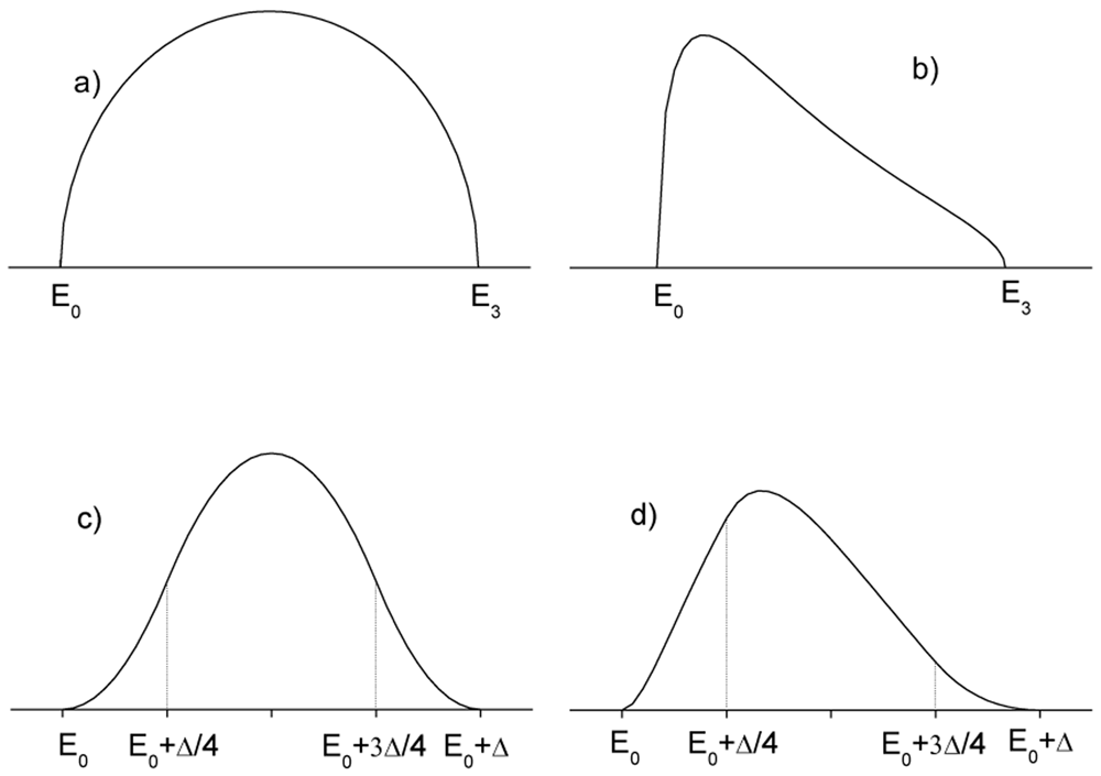
Figure 1.
Imaginary part of the dielectric susceptibility for infinite lifetime semiconductor () and: a) direct gap under Cody’s approximation b) direct gap under Tauc’s approximation, c) indirect gap under Cody’s approximation d) indirect gap under Tauc’s approximation. E0 is the semiconductor gap. The high energy limit of the absorption band is labelled as E3 in a) and b) and as E0 + Δ in c) and d).
On the other hand in Tauc’s approximation, the momentum matrix element is considered independent of energy and therefore, as previously discussed, the transition intensity is proportional to 1/E2 (see Figure 1b), thus:
Other types of critical points do exist (M1 and M2) in the ρ(E)19, but they are not yet included among the fitting functions of kSEMAW.
Both the complex permittivity components for these two cases can be obtained by the convolution between the functions in Equation 12 and Equation 13 and the normalized quantum oscillator .
Direct gap Cody:
where and .
Direct gap Tauc
Different formulas must be used for materials where the fundamental gap is due to indirect transitions: in this case the excitation process includes the absorption or the emission of a phonon necessary to allow transitions between electronic states with different crystalline momentum. The absorption/emission of phonons removes the momentum conservation constraint and therefore for indirect transitions ρ(E) is proportional to the convolution of the density of states of the two bands. In amorphous semiconductors also the momentum conservation is not required because the disorder destroys translational simmetry and momentum is no more a good quantum number. It follows that oscillators for indirect transitions in crystalline semiconductors can be used to fit the optical constants of amorphous semiconductors too.
Analytical expressions for the convolution integral over the whole bands are not available, but it is well known that the convolution between two square root densities of states gives a function which increases parabolically above the gap. Therefore an empirical approximated expression can be obtained by joining two parabolic edges with a parabolic maximum, getting in Cody’s approximation (see Figure 1c):
where E0 is the gap energy and Δ is the absorption band width.
In the Tauc’s approximation the above expressions must be divided by the term E2.
As for the direct gap case, both the complex permittivity components can be obtained by the convolution between these parabolic terms and the normalized quantum oscillator .
Indirect gap-Cody
where:
Where:
Indirect gap-Tauc
where:
where:
Before starting the optimization with the IbridOne method, the function parameters have to be set to initial values good enough to reasonably model n(λ). Then, assuming n(λ), k(λ) values are calculated to perfectly reproduce the T(λ) spectrum; from the knowledge of n(λ) and k(λ), the reflectance spectrum Rcal(λ) and the merit function MF = are calculated. The Levenberg Marquardt non-linear least squares curve fitting (offered by the MINPACK library) is then used to minimize MF optimizing some parameters of the coating model (e.g. thickness) and of the analytical functions used to describe n(λ). Note that when using IbridOne the transmittance spectrum is always perfectly reproduced by construction.
In order to choose the most appropriate analytical functions to be used in IbridOne, at least in the initial phase, it is advisable to launch the tracking method first, to identify the wavelength-behaviour of a physically meaningful solution subset (see use case #1 and #4 as examples). Otherwise, the choice of oscillator functions should be driven by the physical properties of the material under investigation: in this case the oscillator parameters in the Simulation TAB has to be manually adjusted to obtain a first rough reproduction of the experimental curve before launching IbridOne (see use case #5).
In any case, users should never forget that the reliability of the obtained n,k solutions strictly depends on the correctness of the experimental measurements used as input data. We recommend the reading of Appendix B of the user manual which reports some rules of good practice to avoid the most common errors causing artefacts in spectrophotometric measurements.
Prediction of the R and T angular behaviour
Historically, in the first years of its development, kSEMAW was massively used for characterizing architectural glazing: day-lighting and energy consumption evaluation for actual rooms requires knowledge of the luminous and energetic parameters of the fenestration, also at off-normal incidence. The direct experimental measurement of transmittance/reflectance at oblique incidence is very cumbersome: the measurement at a given incidence angle must be separately accomplished for the two light polarizations s and p; several different angles must be considered for sampling the angular range of interest, typically [0,90] deg for architectural glazing and [0,60] deg for the case of Concentrated Solar Power (CSP)23, as well as in Concentrated Photo-Voltaic (CPV).
A simpler approach is offered by the exhaustive optical characterization of the fenestration based on experimental near-normal spectrophotometric measurements and their analysis with a suitable coating optical model. After that, one can numerically evaluate the off-normal incidence behavior24 of any optical features of the device by means of the tools grouped in the Simulation TAB.
Unfortunately, often the multilayer structure of commercial products is undisclosed or it is not perfectly known; therefore further information must be obtained by other techniques25–27, like neutron spectroscopy and ESCA analysis. Anyway, this reverse-engineering process is very difficult and time-consuming.
On the other hand, when the final purpose is the computing of mean values averaged on a standard spectrum, like the energetic and visible parameters of architectural glazing, these mean values are slightly influenced by the realness of the model: as a matter of fact, even if totally unrealistic, optical models perfectly reproducing the experimental measurements at near-normal incidence allow one to predict off-normal incidence features, averaged on solar or visible spectrum, with good accuracy. By virtue of this fact, the Equivalent Model Algorithm (EMA)10 has been proposed. The interested reader will find a detailed discussion and a list of the most useful equivalent models in 10; here we just wish to note that kSEMAW is fully EMA-ready.
The situation in CSP and CPV applications is similar but a bit more complex. Mirrors generally work at off-normal incidence to redirect solar radiation on a receiver. As shown in Figure 2 the solar radiation has an intrinsic divergence (the half-angle is about 5 mrad) and the reflected radiation is captured with the acceptance-angle 2φR of the receiver (typically φR ≤ 20 mrad). Therefore the reflectance relevant for CSP/CPV can be referred to as near-specular, whose value is generally greater than the genuine specular reflectance, strictly related to plane-waves.
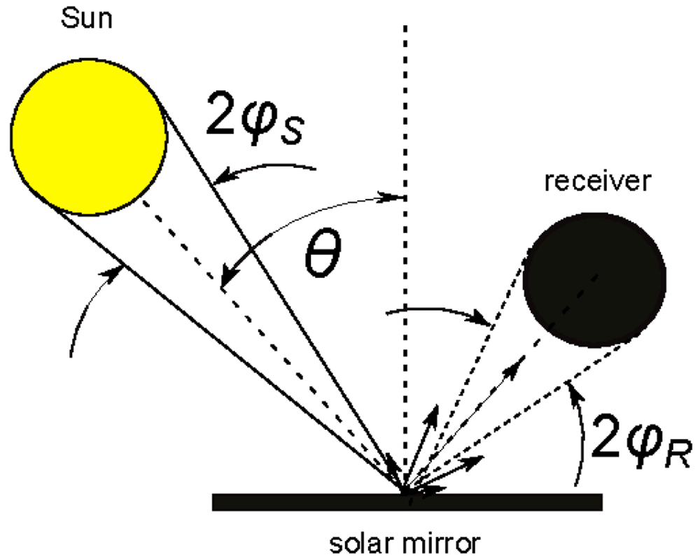
Figure 2. Use case #3: solar mirrors in Concentrated Solar Power (CSP) applications.
Θ is the incidence angle; φS is the half-angle of solar radiation divergence; φR the half acceptance-angle of the receiver.
An international group of experts is drafting the guidelines for reflectance measurement in SolarPACES Task III3. Even if in the latest Reflectance Guideline28 the recommended procedure consists in measuring only the hemispherical reflectance at near-normal incidence, the importance of also measuring near-specular reflectance is now fully acknowledged, but its experimental measurement is a hard task even for highly specialized optics-laboratories because the divergence of the measuring light beam itself may affect the result29.
Strengthened by the experience gained on glass for building, a more reliable general solution based on a new specific Equivalent Model Algorithm for Solar Mirrors (EMA4SM) was recently presented30: EMA4SM represents the latest evolute adaptation of the Equivalent Model Algorithm (EMA)10 to the specific case of solar mirrors with the target of predicting the angular behaviour versus incidence and acceptance angle of the solar-weighted reflectance.
The algorithm EMA4SM needs a few experimental data measured at near normal incidence, such as:
1. hemispherical reflectance spectrum measured in the solar range (320–2500 nm);
2. near-specular or conic reflectance measured at single wavelength and several different acceptance angles in the range of interest.
Considering the high specialization of both the model and the single wavelength experimental measurements, we have decided to separate this functionality from kSEMAW and arrange the new software SMQexpo for dealing the specific case of solar mirrors. Such software embraces the Open Source philosophy and is freely distributed; interested people can request it by sending an email to marco.montecchi@enea.it.
Therefore actually kSEMAW can be only used for highly specular solar mirrors, i.e. in the cases where near-specular reflectance is equal to the specular one, within the experimental error.
Implementation and operation
Referring to the user manual for installation details, here we just note that we use to install kSEMAW on PC with Linux operative system (Manjaro or Debian distro). For MS Windows users, dual booting or the installation in a Linux virtual machine are the recommended ways to get kSEMAW working, although in principle the software could be directly installed in Windows and IOS PCs, but we never tried that.
kSEMAW consists of two executables. The first, named ksemaw, C++ written, and based on Qt libraries, manages the graphical user interface (GUI) for data input-output. The second one, named ksemawf, FORTRAN written, runs in background and executes the required computing.
The FORTRAN executable requires the two libraries MINPACK and pgplot.
In order to harmonize the MINPACK sources with the GNU FORTRAN compiler gfortran, a slightly modified version is added to kSEMAW sources; that complies with the MINPACK disclaimer.
The library pgplot is offered as a binary package in most of LINUX distros. As declared in the copyright: “PGPLOT is not public-domain software. However, it is freely available for non-commercial use”, like in the case of kSEMAW.
The C++ executable is devoted to control the Graphical User Interface (GUI), which is based on the open source version of the Qt library, which is offered as binary packages in any LINUX distro.
When launched, two windows pop-up: the GUI and a Linux terminal; the latter shows the progress of the workflow in the two executable C++ (ksemaw) and FORTRAN (ksemawf); messages from C++ are preceded by “->”.
The two executable interact by means of the two text files ksemaw.ctrl and defau.1.Spj: the former contains the imparted command or the process status, the latter the full parameter set characterizing the current project. Figure 3 describes the workflow at the launch of a given command from the GUI. Once the imparted task has been completed, the FORTRAN executable writes “p” in the file ksemaw.ctrl; the executable C++, alerted for the modification of that file, once found “p”, reloads defau.1.Spj which in the meanwhile has been refreshed by ksemawf. A scheme of the workflow is depicted in Figure 3
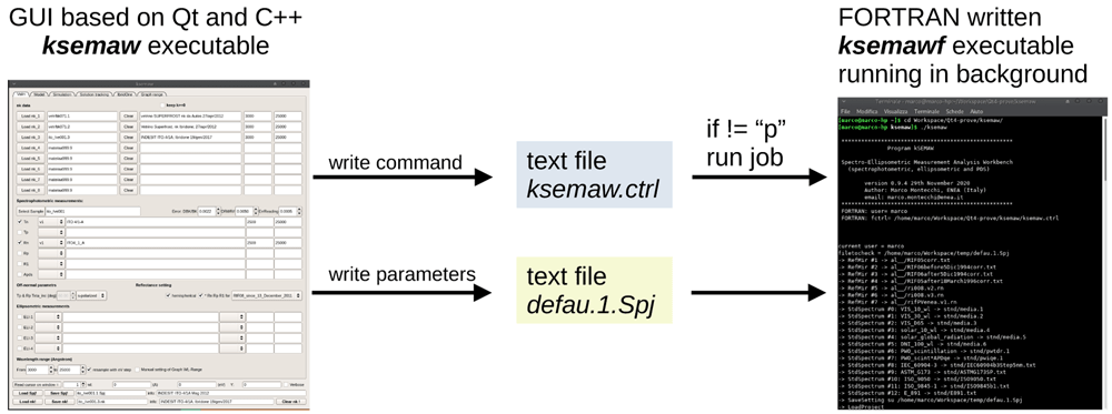
Figure 3. Workflow at the launch of a given command from the kSEMAW graphical user interface.
The GUI, shown in Figure 4, is composed by a top part, structured in 6 “tabs”, ordered in logical sequence, and a bottom part, always visible.
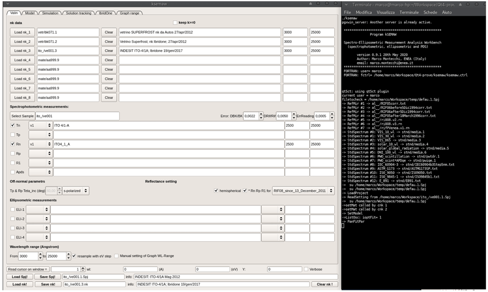
Figure 4. Graphical interface and terminal of kSEMAW.
The 6 TABs are:
1. Valin: selection of nk-files and measurements to be imported in the analysis work bench.
2. Model: setting of the optical device model.
3. Simulation: simulation of measurements on the basis of known (n, k).
4. Solution tracking: (nλ, kλ) solution search in tracking mode in the spaces (λ, n) and (λ, k).
5. IbridOne: iterative procedure:
step-1: n(λ) model
step-2: k(λ) computing from T(λ) given n(λ)
step-3: best-fit of R(λ) with n = n(λ, p1, p2,..., pM) by close loop on these 3 steps.
6. Graph range: management of XY plots
The bottom part, always visible, contains
reading of the cursor position on one of the opened windows
loading/saving the SEMAW project file (.Spj)
loading/saving the file with the solutions nλ, kλ (.nk)