Plain language summary
This paper examines the effect of financial development, measured by broad money, domestic credit, and mobile money, on poverty and human development in the Southeast Asian economies, using the dataset from 1990 to 2017. The findings suggest that broad money and domestic credit contribute to poverty reduction and promote human development. The role of mobile money is seen to have a statistically positive impact only if we analyse it with human development. Additionally, when we take a closer look at the different stage of economic, political, and institutional development in this region, we found that the positive effect of broad money and domestic credit is mostly found only in the less developed and less democratic countries. The mobile money, on the other hand, is found to statistically promote the human development in both groups of countries, but there is no statistical relationship for poverty analysis.
Introduction
The Sustainable Development Goals (SDGs) (https://www.undp.org/sustainable-development-goals) of the United Nations (UN) aim to leave no one behind by 2030, along with achieving a better and more sustainable future for all (UN, 2019). We, from a community to a country or the region to the whole world, are facing many global challenges, especially those related to reducing poverty and promoting human development. To achieve these ambitious goals, it is, without doubt, a matter for all states in every corner around the globe. Therefore, searching root causes to attain the SDGs in sub-regional context is always significant, and there is no exception for the Southeast Asian countries.
Along with many priorities, promoting financial development and financial technology is one of the most significant policies to accomplish the promise. Precisely, the World Bank1 states that “financial development reduces poverty and inequality by broadening access to finance to the poor and vulnerable groups, facilitating risk management by reducing their vulnerability to shocks, and increasing investment and productivity that result in higher income generation” (World Bank, 2019). Alternatively, the development of financial technology or digital finance revolution - through for instance, the introduction of mobile money - alone contributes directly to 13 of the 17 SDGs by, for example, providing financial services to individuals and small businesses that would otherwise be financially excluded; enabling access to electricity, water, and sanitation (e.g. via mobile pay-as-you-go solutions); facilitating access to low-cost remittances; providing means for parents to pay school fees; and by facilitating cash transfers during emergencies (Ramos & Steiner, 2019).
Economic theory provides a wide range of explanations for the potential impact of financial development and financial technology on poverty and human development. Theories identifying the positive effects are often associated with theories through economic growth, job creation, investment, and optimal allocation of capital. There is evidence suggesting that “financial sector development plays a huge role in economic development. It promotes economic growth through capital accumulation and technological progress by increasing the savings rate, mobilizing and pooling savings, producing information about investment, facilitating and encouraging the inflows of foreign capital, as well as optimizing the allocation of capital” (World Bank, 2019). These results are in accord with recent studies indicating that financial development reduces poverty and inequality along with promoting human development because it may help the poor and the most vulnerable by access to finance, improving their business or investment, and reducing uncertainty in case if they face any economic shocks (Demirgüç-Kunt et al., 2013; Kiendrebeogo & Minea, 2016; Rewilak, 2017; Uddin et al., 2014). Financial sector development is also found to promote the SMEs, increasing job creation, and ameliorating labour productivity in emerging economies (Banerjee et al., 2015; Bekaert et al., 2011; Kaboski & Townsend, 2012; Karlan & Zinman, 2010). Cai & Treisman (2005) explain how competition for capital disciplines governments in the context of decentralization, globalisation, and public policy. However, finance is good for the poor, but it depends where they live (Rewilak, 2013) and how they relationally use it (Chhorn, 2020).
The existing literature emphasizes the positive effect of financial technology in many different ways. The technological progress expects not only to extend financial products and services to excluded households living in a rural area, but also to involve in innovating a new wide range of financial products and services including savings, transactions, payment, and insurance (Kangni & Mihasonirina, 2011; Peterson, 2018; Shem et al., 2017). In many cases, financial technologies such as ‘mobile money’ open novel and exciting possibilities for democratizing monetary and financial inclusion. The poor do not always behave as technologies anticipate, but actively reshape monetary spaces through innovations such as informal money transfer mechanisms (Atika, 2018; Daniela & Sally, 2017). Digital finance and financial inclusion have several benefits to financial services users, digital finance providers, governments and the economy such as increasing access to finance among poor individuals, reducing the cost of financial intermediation for banks and FinTech providers, and rising aggregate expenditure for governments (Peterson, 2018; Vighneswara, 2014). Mobile money refers to a suite of financial services offered through mobile phones and other handheld mobile devices. These services can include mobile banking, through which customers can access their bank accounts, pay bills, or deposit and withdraw funds (Dolan, 2009). Mobile technology may help engender inclusive development, reduce inequality, increase income, facilitate cooperation and information sharing, among others (Joshua et al., 2018). It is because mobile phones reduce information search costs and enable villagers to have access to the weather, market and price information, all of which will support production and productivity.
Several theories depict, however, the adverse effect that financial development and financial technology negatively affect the economy through instability, sharing crisis, transmission of political risk or rising inequality. The rise of financial development within a country may also indicate that the country has opened to the rest of the world, through for example cross-border capital flows. This can be a source of economic instability, a magnifier of distortions, and international risk sharing, especially those from advanced countries to developing countries (Cole & Obstfeld, 1991; Wei, 2018). The developing countries that were affected badly during the global financial crisis in 2009 can be empirical evidence in this case. Alternatively, financial development may boost economic growth at the first stage of economic development, but also leave rising inequality, i.e., the fruits of economic growth might go only to those in the top income bracket and those living in urban areas, mainly in developing countries. Inequality adversely affects economic growth in the latter stage. The relationship on how income distribution affects poverty can be found in the poverty-growth-inequality (PGI) triangle of Bourguignon (2004). This outcome is consistent with empirical studies in the US and Europe by Demirgüç-Kunt et al. (2013). Therefore, the economic distortion may hurt the poor and human development in the long run.
Another aspect of studying the effect of financial development on poverty and human development is to consider other factors in explaining this relationship. It suggested that the impact of financial development depends on the level of growth, productivity, domestic savings, and the quality of institutions (Broner & Ventura, 2016). The countries, which are more corrupted and have weaker public governance, are likely to be systematically less attractive to foreign direct investment (FDI), less favourable for equity investment from international institutional investors (mutual funds, pension funds, and hedge funds), and have more external debt (Gelos & Wei, 2005; Tong & Wei, 2011). If the domestic financial system is less efficient and distorted, receiving finance from the outside can lead to misallocation of resources. In this regard, countries, especially from the developing world, cannot benefit from financial development if they have these key challenges, including distortions in the domestic labour market or weakness in local governance institutions (Eichengreen & Leblang, 2003; Ju & Wei, 2010).
Therefore, considering the implication of financial development and financial technology on poverty and human development, we address the following questions from an empirical perspective. The goal of this paper is to improve our understanding of this association and its implications for Southeast Asian countries:
- First, how does financial development and financial technology affect poverty and human development in Southeast Asian countries?
- Second, what are the political and institutional factors that shape financial development and financial technology, considering a vast difference in political systems in Southeast Asian countries?
This paper contributes to the literature in many ways. First, we introduce financial technology, measured by the development of mobile money, through a macroeconomic viewpoint in the analysis. Second, it focuses on the Southeast Asian countries, which are a relatively heterogeneous sample, over two decades from 1990 to 2017. Third, it establishes the extent to which financial development and financial technology drive poverty and human development in the region, using instrumental variables panel data estimations that include numerous control variables.
The next section starts with the discussion of stylized facts in Southeast Asian countries. The methods section explores the empirical methodology of this study with the construction of our measure, regression model, and robustness, followed by our results and discussion sections which includes the robustness checks.
Stylized facts of the Southeast Asian nations
The Southeast Asian region is home of 10 independent countries: Brunei Darussalam, Cambodia, Indonesia, Lao PDR, Malaysia, Myanmar, the Philippines, Singapore, Thailand, and Vietnam. In 1967, the regional community, namely the Association of Southeast Asian Nations (ASEAN), originated by five founding members, and, as of 1995, another five members joined the community, making ten member states in total. With more than 630 million people, the ASEAN is the World’s fourth-largest market behind China, India and the EU. Their combined economies are worth USD 2.555 trillion in the nominal term, the World’s fifth largest economies behind the USA, the EU, China and Japan.2 The region is seen as the second most successful community beside the EU and geographically regarded as the heart of the world’s 21st century (Mahbubani & Sng, 2017). That is the reason why we might see countless economic and political meetings in this region between the global superpowers, including the EU, the USA, China, Japan, and India. Asian leading scholar Sir Kishore Mahbubani, one of the top 100 global thinkers by Foreign Policy in 2005, 2010, and 2011 and one of the top 50 world thinkers by Prospect Magazine in 2014, stated that whenever the global superpowers cannot find where to talk or what occasion to meet each other, Southeast Asia is the most strategic or the last resort place for them (Mahbubani & Sng, 2017). To give the most recent example, Singapore and Vietnam were chosen respectively to host the 2018 and 2019 North Korea–United States Summits. It argued that whenever this region prospers, it would be more significant for global cooperation and economic development.
In this study, we include only the eight Southeast Asian countries: Cambodia, Indonesia, Lao PDR, Malaysia, Myanmar, the Philippines, Thailand, and Vietnam. Brunei Darussalam and Singapore were not included because these two countries are the wealthiest states in the region and have GDP (purchase power parity (PPP)) per capita3 of USD 81,612 and USD 98,255 respectively. This income level is comparable to those of the first world; therefore, it is nonsense to examine the poverty of these two countries. This section focuses on the descriptive dynamics of poverty, human development, financial development, and financial innovation.
Poverty and human development
Figure 1 and Figure 2 show that extreme poverty in Southeast Asia has significantly reduced while the human development index has dramatically improved during the last three decades. Two groups of countries should be notified in the region, considering the analysis of poverty and human development. The five founding members of ASEAN are always the most developed nations in terms of per capita GDP and human development. However, Cambodia, Lao PDR, Myanmar and Vietnam (CLMV), are the most impoverished nations.
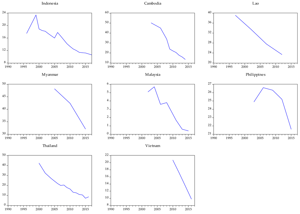
Figure 1. Poverty headcount ratio at national poverty lines (% of population) 1990–2017.
Source: World Bank, Global Poverty Working Group. Data are compiled from official government sources or are computed by World Bank staff using national (i.e., country–specific) poverty lines.
https://databank.worldbank.org/source/world-development-indicators.
Notes: The graphic was built by using the national poverty headcount ratio with xtline command in STATA. The detail of the database definitions, sources, links, ID, license, date of access, and duration is shown in the Methods section. In our research, there are many missing values for poverty variable which includes some missing years in the above figure. It represents less than 30% values among the full 224 observations for poverty.
In 1990, around half the population in sub-saharan Africa and Asia were living on less than US $1.25 purchase power parity (PPP) per day. In 2015, the rate was reduced to well below 20% in Asia while in sub-saharan Africa, it remains relatively high at around 40% (ASEAN Secretariat, 2017). As shown in Figure 1, since the early 2000s, the poverty rate in Southeast Asian countries has decreased dramatically, except the Philippines, where poverty has varied around 20% of the total population. With the lowest rate, Malaysia’s poverty was about 5% in the early 2000s and decreased to 0.4% in 2015. Myanmar, with a population of more than 50 million, is the home of poverty. Its poverty rate is presently 30% of the total population, i.e., the highest percentage among other member countries. According to the UN (2017), poverty reduction is the highest in the priority list and an essential goal in the development plans of most countries in this sub-region.
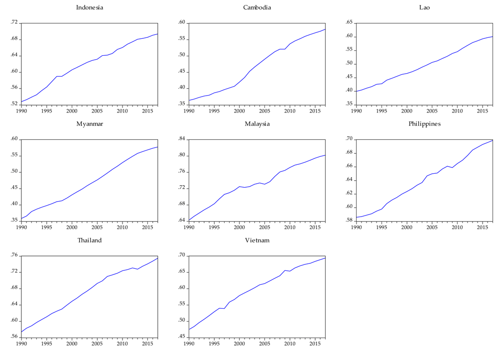
Figure 2. Human development index (HDI) 1990–2017.
Source: The UN Development Programme (UNDP) Human Development Reports. Statistical references relate to statistical material presented in this Statistical Annex and in the full set of statistical tables posted at http://hdr.undp.org/en/human-development-report-2020.
Notes:The graphic was built by using the HDI with xtline command in STATA. The detail of the database definitions, sources, links, ID, license, date of access, and duration is shown in the Methods section. The unit of measurement of HDI is as follows: 0.800–1.000 (very high human development), 0.700–0.799 (high human development), 0.550–0.699 (medium human development), and 0.350–0.549 (low human development).
The Millennium Development Goals (MDG) by 2015 aimed to halve global poverty (Besley & Burgess, 2003). However, the SDG by 2030 aimed to have no poverty. The SDG 2030 agenda states that ”this agenda is a plan of action for people, planet and prosperity. It also seeks to strengthen universal peace in larger freedom. We recognize that eradicating poverty in all its forms and dimensions, including extreme poverty, is the greatest global challenge and an indispensable requirement for sustainable development.”4
The HDI has increased in an almost linear trend in every country since the 1990s. Countries with higher national income have a relatively higher score of HDI. In the Southeast Asian countries, Vietnam’s HDI, despite being classed among the CLMV countries, is ranked among the more developed countries, including Malaysia, Thailand, the Philippines, and Indonesia.
Financial development and financial crises
Figure 3 and Figure 4 report the dynamic trend of financial development variables, measured by broad money (% of GDP) and domestic credit provided by the financial sectors (% of GDP), in the Southeast Asian countries from 1990 to 2017. During this particular period of time, this region experienced two major financial crises; the Asian financial crisis in 1997 and the global financial crisis from 2007 to 2009.
We can observe an overall rising trend of broad money (% of GDP) in almost all countries, except Indonesia, where its trend has remained around 45%. Vietnam’s broad money (% of GDP) has increased impressively, from one of the smallest shares in the early 1990s to be one of the highest percentages among top groups, including Malaysia and Thailand. Cambodia and the Philippines are in the group whose rate is among the higher average, above Myanmar, Indonesia and Laos.
The domestic credit (% of GDP) in Vietnam also shows impressive increasing trends. This country started from one of the lowest domestic credits to one of the highest percentages of GDP in the Southeast Asian countries. Overall, we can separate the sampling into two groups of countries: the group with the higher percentage (Thailand, Malaysia, and Vietnam) and group with the lower percentage (the rest of the countries). Thailand, Malaysia, and Vietnam are moving toward the same group with its share of GDP as very high, moving around/towards 150% of GDP. Other countries have varied below 100% and some around 50%.
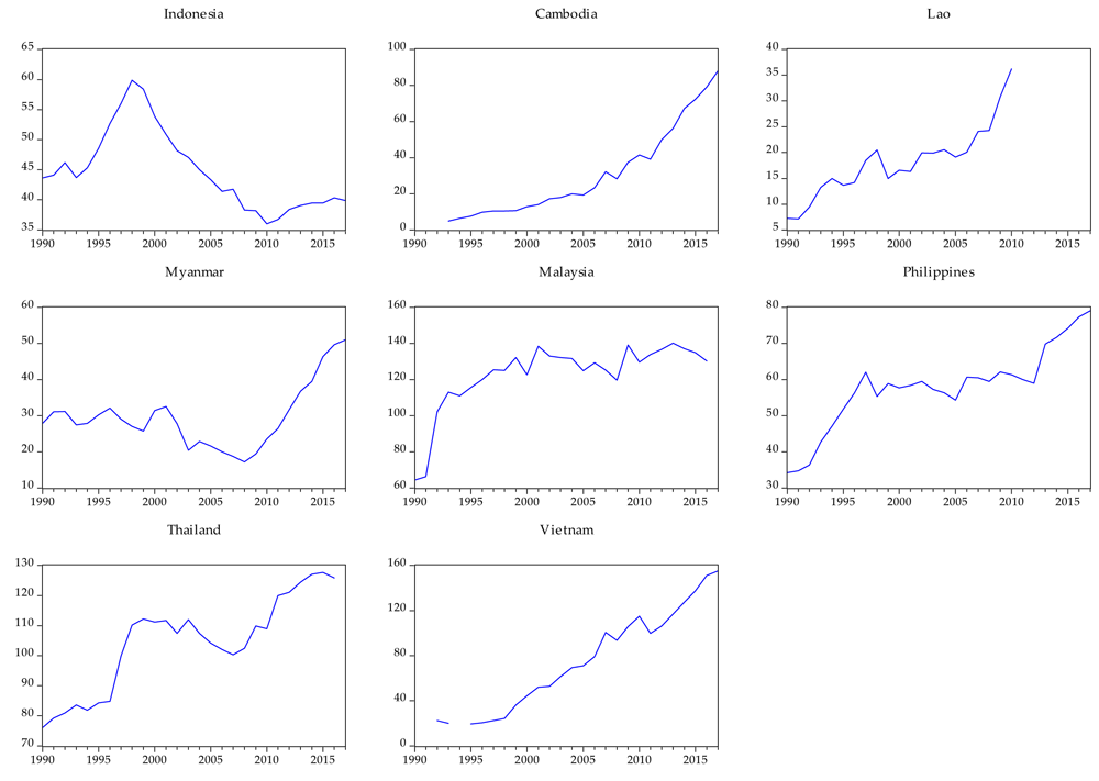
Figure 3. Broad money (% of GDP) of the Southeast Asian nations 1990–2017.
Source: International Monetary Fund, International Financial Statistics and data files, and World Bank and OECD GDP estimates. https://databank.worldbank.org/source/world-development-indicators.
Notes: The graphic was built by using the IDN Broad money (IFS line 35L..ZK) with xtline command in STATA. The detail of the database definitions, sources, links, ID, license, date of access, and duration is shown in the Methods section.
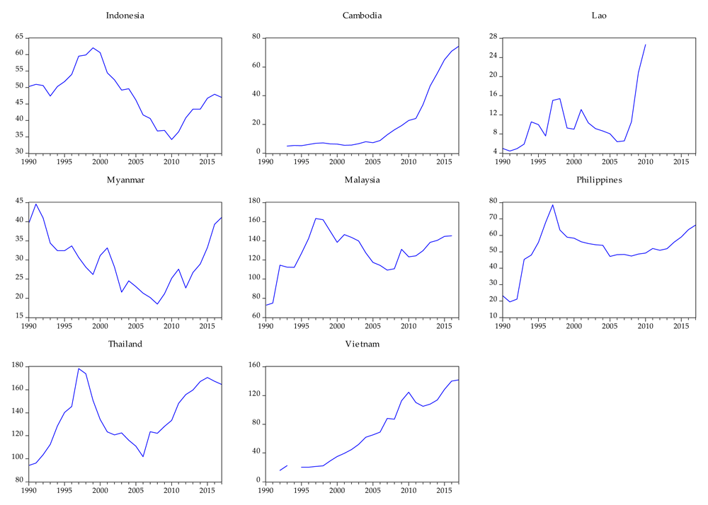
Figure 4. Domestic credit provided by financial sector (% of GDP) of the Southeast Asian nations, 1990–2017.
Source: International Monetary Fund, International Financial Statistics and data files, and World Bank and OECD GDP estimates. https://databank.worldbank.org/source/world-development-indicators.
Notes: The graphic was built by using the domestic credit provided by the financial sector (% of GDP) with xtline command in STATA. The detail of the database definitions, sources, links, ID, license, date of access, and duration is shown in the Methods section.
Financial technology
To contribute to the literature in studying the role of financial technology, we include the existence of mobile cellular subscriptions and mobile money in the analysis. Unlike advanced economies, where financial sectors are developed and many people can access its services and products, the financial sectors in developing countries, like those in Southeast Asia, are still by far only accessed by higher-income citizens and those living in urban and capital cities. However, the favourable socio-demographic trends combined in the Southeast Asian countries with recent developments in financial technology and mobile banking have seen as the driving force that could support initiatives aiming at providing financial services to the most vulnerable groups. The use of technology in the banking sector contributes to more efficient risk management and helps reduce operational costs, which should make banking products and services more affordable for the poor. In this regard, the mobile phone which is held by more people from lower-income backgrounds and living in rural areas can be a solution for developing countries. In one perspective, it might help to deal with the poverty issue, but in other aspects, it might also be interesting to deal with human development issues.
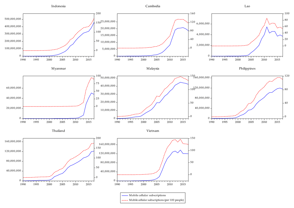
Figure 5. Mobile cellular subscriptions (per 100 people), 1990–2017.
Source: International Telecommunication Union ( ITU ) World Telecommunication/ICT Indicators Database. https://databank.worldbank.org/source/world-development-indicators.
Notes: The graphic was built by using the mobile cellular telephone subscriptions with xtline command in STATA. The detail of the database definitions, sources, links, ID, license, date of access, and duration is shown in the Methods section.
Figure 5 indicates that nearly every person among the 100 people sample had no mobile phone in the 1990s; however, by 2017 more than 100 or 150 mobiles have been presently held by 100 people, except in Myanmar and Laos, where mobile phone holders are less than 100.
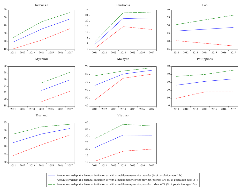
Figure 6. Account ownership at a financial institution or with a mobile-money-service provider (% of population ages 15+) 2011–2017.
Source: The Economist, 2018, Global Financial Inclusion Database, World Bank. https://databank.worldbank.org/source/world-development-indicators. Notes: The graphic was built by using the account ownership at a financial institution or with a mobile-money-service provider (% of population ages 15+) with xtline command in STATA. The detail of the database definitions, sources, links, ID, license, date of access, and duration is shown in the Methods section. The dataset of the mobile money was available only in 2011, 2014, and 2017.
Figure 6 shows the account ownership at a financial institution or with a mobile-money-service provider (% of population aged 15+) in the Southeast Asian countries from 2011 to 2017. Up to the present, nearly every person is holding at least one mobile phone, and some are holding more than one mobile phone, but only Malaysian and Thai people, who the account ownership at a financial institution or with a mobile-money-service provider with the percentage of about 80% of the total population. It is the highest percentage among the member countries. Other countries have their rate, varying between 20% and 50%.
Methods
Data collection
We collected data from 1990 to 2017 in the eight Southeast Asian countries: Cambodia, Indonesia, Lao PDR, Malaysia, Myanmar, the Philippines, Thailand, and Vietnam from various sources: Eurostat: Demographic Statistics, Global Financial Inclusion Database, World Bank, Government Finance Statistics Yearbook, International Financial Statistics, International Labour Organization, ILOSTAT database, International Monetary Fund, International Telecommunication Union (ITU), Organisation for Economic Co-operation and Development (OECD), Secretariat of the Pacific Community: Statistics and Demography Programme, the UN Development Programme (UNDP) Human Development Reports, U.S. Census Bureau: International Database, UN Statistical Division, World Bank, Global Poverty Working Group, World Bank, World Development Indicators, World Population Prospects: 2019 Revision, and World Telecommunication/ICT Indicators Database. Appendix 1 describes the database definitions, sources, links, ID, license, date of access, and duration. In our research, there are many missing values for poverty variable. It represents less than 30% values among the full 224 observations for poverty.
Equation model. We investigate poverty and human development, linking to financial development and financial technology variables by including many additional control variables into the analysis. The annual data are taken from the eight Southeast Asian countries from 1990 to 2017 as outlined in the data collection section. The equation indicates our overall regression model, using the instrumental variables and fixed-effects two-stage least squares for panel-data models (IV-FE2SLS).
Where is the dependent variable from the fixed-effects model, explaining respectively poverty and human development, of country i at time t. It should note that we estimate our model for poverty and human development separately; therefore, there is no relationship between these two dependent variables. α is constant. is the lagged dependent variable. is the proxy of the explanatory variables from the fixed-effects model, which is built with the instrumental variables. This proxy includes the financial development variable (measured by broad money as % of GDP and domestic credit provided by financial sectors as % of GDP), and the financial technology variables (measured by mobile cellular subscriptions per 100 people and account ownership at a financial institution or with a mobile-money-service provider as % of population ages 15+). are additional control variables, including GDP growth (annual %), government expense (% of GDP), inflation consumer prices (annual %), and population growth (annual %). ui is the country fixed effect to control unobserved cross-country heterogeneity. yt is the time fixed effect to control the Asian financial crisis in 1997 and global financial crises during 2007 to 2009. εit is error term.
The following is a detailed explanation on how we build our model. We start by constructing the following equation for each country:
From the Equation (2), if we set the boundary of our analysis to only time-varying covariates and we assume that all the variables are truly exogenous, we may apply the one-stage least square estimations. However, there are many statistical issues, which we have to critically consider in order to obtain good estimations and will address in further detail below. To deal with this issue, we use instrumental variables and fixed-effects two-stage least squares for panel-data models. Staehr (2018) uses the country fixed effect model to study the relationship between capital flows and growth dynamics in 11 post-communist Central and Eastern Europe with the dataset from 1995 to 2015. We use instrumental variables in the two-stage least square panel-data estimations to avoid any endogeneity bias, driven by the fact that the variables in our analysis are not exogenous.
Firstly, one statistical problem that may occur from the Equation (2) is related to the exclusion of the lagged dependent variable Yit – 1. In the macroeconomic literature, the dependent variable Yit is normally affected by its past value (Fatás & Mihov, 2003). We introduce, therefore, the lagged poverty and human development (–1) to take into consideration unexplained factors of poverty and human development. This is another problem which may also arise because the addition of the lagged Yit–1 can produce biased results from the fixed effects estimations (Nickell, 1981). However, if we have a small number of cross-sections and the outcomes of autoregressive coefficients are modest, the biased results are relatively small and reasonable (Anderson & Hsiao, 1981). Thus, the results from fixed-effects estimations are somehow more reliable than the System Generalized Method of Moments (GMM) estimators (Bun & Kiviet, 2001; Judson & Owen, 1999). In our studies, since we cannot obtain accurate and satisfying results, we decide not to show the estimation with lagged analysis.
Secondly, it is related to the problem of causality, which we use to identify cause and effect, as what we hope to get is only the causal direction from the explanatory variable financeit to the dependent variable Yit and not vice versa. The idea is to remove variation in explanatory variables financeit that may be caused by the dependent variable Yit. We then keep the part of financeit, which is not explained by Yit. In this regard, we need to find the instrumental variable and/or variables Z that is/are correlated with financeit, but not with error term, which is an unexplained part of financeit (Deaton, 2019).
In this study, the instrumental variables include total natural resources rents (% of GDP), employment in agriculture (% of total employment), and rural population (% of the total population). It suggested that developing or poor countries typically have a high percentage of rural households and a high proportion of agricultural employment. Although these countries are rich in natural resources but have weak institutions and high corruption, the financial sector in those countries tends to be less developed.
According to Bhattacharyya & Hodler (2014), natural resource revenues may deteriorate contract enforcement if political institutions are weak. As poor contract enforcement leads to low financial development, resource revenues may hinder financial development in countries with weak political institutions, but not in countries with comparatively better political institutions. Acemoglu et al. (2001) explain that the states, which are rich in natural resources and have weak governance, typically design their institutions only to support the political powers. In their study on the politics of financial development in many countries in the twentieth century, Rajan & Zingales (2003) suggest that political powerful elites might restrict financial development from new firms’ competition for their own personal interest because the new firms might danger the existing dominant firm institutions. Therefore, we would expect less financial development in those countries.
At the first stage we estimate financeit by the instrumental variables. We obtain the following equation:
Estimate: financeit = α + βZit + ξit
Compute predicted value: = α + βZit
The instrumental variables are valid only if the following assumptions are respected: (a) the exclusion restriction is: E[ε|Z] = 0 → Zit does not explain directly, but only through financeit. In this case, Zit is exogenous with regards to Yit; (b) the relevance is: Cov(financeit,Zit) # 0. It is important to take note that if Zit is a valid instrument, then financeit does not ‘contain’ effect from Yit to financeit, but it reflects part of financeit, which is exogenous with regards to Yit. Murray (2006) explains how to avoid invalid instruments and cope with weak instruments. More precisely, for the validity of the instruments, we use the first-stage F-statistic. If its statistical value is bigger than 10, we assume therefore that the model has good instruments. In the same way, we use the Sargan-Hansen test of overidentification of restrictions of instruments. If the p – value is bigger than 5%, we assume that there is a non-rejection of the null hypothesis. Therefore, we obtain good instruments from this test.
At the second stage, we estimate the Equation (2) with our predicted value of explanatory variables. Therefore, our regression equation becomes as follows:
In Equation (3), the estimation of β in principle is consistent, reflecting effect from to Yit. Yet, it is less efficient if standard error (SE) is larger.
From the results of the pairwise correlation between instruments and explanatory variables in Table 1, we observe that there are significantly high correlations between employment in agriculture and the rural population to almost all financial development and financial technology variables. Therefore, we might expect good instruments. However, natural resources seem to be correlated at a very weak coefficient with almost explanatory variables. It is required to detect it carefully and interpret with very high caution.
Table 1. Pairwise correlation between instruments and explanatory variables.
| NR | EA | RP | M2 | DC | MOBILE | MOBILE_$ |
|---|
| NR | 1 | | | | | | |
| (Sig. 1%) | | | | | | | |
|
Nb. of Obs.
| 203 | | | | | | |
| EA | 0.081 | 1 | | | | | |
|
(Sig. 1%)
| (0.259) | | | | | | |
|
Nb. of Obs.
| 197 | 216 | | | | | |
| RP | -0.091 | 0.875*** | 1 | | | | |
|
(Sig. 1%)
| (0.197) | (0.000) | | | | | |
|
Nb. of Obs.
| 203 | 216 | 224 | | | | |
| M2 | -0.021 | -0.774*** | -0.662*** | 1 | | | |
|
(Sig. 1%)
| (0.773) | (0.000) | (0.000) | | | | |
|
Nb. of Obs.
| 194 | 203 | 209 | 209 | | | |
| DC | -0.080 | -0.697*** | -0.608*** | 0.954*** | 1 | | |
|
(Sig. 1%)
| (0.267) | (0.000) | (0.000) | (0.000) | | | |
|
Nb. of Obs.
| 194 | 204 | 210 | 209 | 210 | | |
| MOBILE | -0.106 | -0.578*** | -0.458*** | 0.543*** | 0.450*** | 1 | |
|
(Sig. 1%)
| (0.132) | (0.000) | (0.000) | (0.000) | (0.000) | | |
|
Nb. of Obs.
| 203 | 216 | 224 | 209 | 210 | 224 | |
| MOBILE_$ | -0.121 | -0.557*** | -0.768*** | 0.598*** | 0.781*** | 0.547*** | 1 |
|
(Sig. 1%)
| (0.680) | (0.007) | (0.000) | (0.009) | (0.000) | (0.009) | |
|
Nb. of Obs.
| 14 | 22 | 22 | 18 | 19 | 22 | 22 |
Thirdly, it is related to the problem of the omitted variables (that we might forget to include one of the relevant explanatory variables) and multicollinearity (that these variables might highly correlate with each other). We, therefore, include several significant additional control variables, which are theoretically linked to poverty and human development. These variables include GDP growth (annual %), government expense (% of GDP), inflation consumer prices (annual %), and population growth (annual %). Trade (% of GDP) and labour force participation rate are also in our consideration to include in additional control variables; nevertheless, we decide to drop these variables because these variables are highly correlated to others. The trending of additional control variables are available in the extended data appendices 2–10 (Chhorn, 2021).
From the results of pairwise correlation between additional control variables in Table 2, we confirm that the problem of having multicollinearity should be avoided as the highest coefficient is -0.442 between expense (% of GDP) and GDP growth.
Table 2. Pairwise correlation between additional control variables.
| GDP | EXP | INF | POP |
|---|
| GDP growth (annual %) | 1 | | | |
|
(Sig. 1%)
| | | | |
|
Number of observations
| 220 | | | |
| Government expense (% of GDP) | -0.442*** | 1 | | |
|
(Sig. 1%)
| (0.000) | | | |
|
Number of observations
| 135 | 135 | | |
| Inflation consumer prices (annual %) | -0.039 | -0.209 | 1 | |
|
(Sig. 1%)
| (0.573) | (0.015) | | |
|
Number of observations
| 213 | 135 | 213 | |
| Population growth (annual %) | -0.157 | 0.006 | 0.013 | 1 |
|
(Sig. 1%)
| (0.020) | (0.948) | (0.847) | |
|
Number of observations
| 220 | 135 | 213 | 224 |
We include therefore the additional control variable into the regression equation:
To estimate the coefficients β and η of financial development, financial technology and additional control variables in Equation (4), the fixed-effects model follows the within transformation (StataCorp, 2013). The within transformation of a variable, for example finance, is:
Where,
Where n and N are the number of groups and the total number of observations of the variable, respectively. The within transformation of Equation (4) becomes therefore:
The model removes the ui (country fixed effects or time-invariant covariate as it is varying with country but not, for example, time, race, or membership year in ASEAN community of any Southeast Asian countries). Then, we can estimate with the two-stage least-square regression (2SLS) of dependent variables () on explanatory variables with instrumental variable ().
Let’s suppose that we have constant and k variables, then, the parameters of the model are k + n – 1, and the conventional VCE for the within estimator is:
Where VIV represents the VCE from the 2SLS.
From the estimated results, we obtain therefore: The is its standard deviation and its correlation with . The εit is the regression’s estimated root mean squared error that is adjusted for the n – 1 estimated means. With the null hypothesis indicating that is different from zero, the estimated results from the regression also report F Statistics (Wooldridge, 1990).
- R2 is calculated as the R2 from the mean-deviated regression
- R2 is calculated as {corr(,)}2
- R2 is calculated as {corr(,)}2
Finally, it is related to the way we interpret the results. We can interpret the coefficient of all variables only as deviation from their country mean. It explains within-dynamic of individuals, but not differences between individuals, i.e., it does explain to what extent Yit differs from , but it does not explain why is different from (Hsiao, 2010; Mundlak, 1978). In this model, the coefficient of variables is identified only through the within dimension of the data. We cannot therefore estimate the coefficient of time-invariant individual variables such as birth year of membership in ASEAN community, race, etc. We can only estimate by interacting time-invariant variables with time dummies and estimate the variable-in-time effect.
Results
Estimating the effect of financial development on poverty and human development
We start our regression of financial development variables on poverty and human development, also including country fixed effects and dummies of the Asian financial crises in 1997 and the global financial crises from 2007 to 2009. The impact of financial crises on poverty and human development can be found in the following empirical and theoretical works (Fiorentini, 2015; Jarrow, 2014; Mohseni-Cheraghlou, 2016; Nikoloski, 2011). The specific experiences of the Southeast Asian countries and the Asian and global financial crises are also examined (Knowles et al., 1999; Rasiah et al., 2014).
We then introduce the additional control variables, including GDP growth (annual %), government expense (% of GDP), inflation consumer prices (annual %), and population growth (annual %), into the analysis. Finally, we estimate the specification with instrumental variables and two-stage least squares for panel-data models. To eliminate the possibility that the dependent variable drives the instrumental variables itself, we include the following instruments, including total natural resources rents (% of GDP), employment in agriculture (% of total employment) and rural population (% of the total population). The data in parentheses () indicates standard errors. P–value, where *** p < 0.01, ** p < 0.05, and * p < 0.1 denote significance levels. At the bottom of the regression results, the table shows First stage F stat, which is used to test for weak instruments. In case if p – value of First stage F stat is smaller than 5%, we obtain good instruments. Since most of the variables are estimated in logs, the coefficients are interpreted as elasticity from an economic point of view.
Table 3 presents the formal regression analysis between financial development variables, using broad money (% of GDP), and domestic credit provided by the financial sectors (% of GDP), on the poverty and human development with the dataset from 1990 to 2017 in the Southeast Asian countries.
Table 3. Fixed-effect estimations of the poverty and human development with additional control variables.
| (POV3.1) | (POV3.2) | (HDI3.1) | (HDI3.2) |
|---|
| Broad money | -0.716** | | 0.038*** | |
| (% of GDP) | (0.352) | | (0.010) | |
Domestic credit provided by financial
sectors (% of GDP) | | -0.527** | | 0.025*** |
| (0.205) | | (0.006) |
| GDP growth | -0.082 | -0.081 | 0.008* | 0.008* |
| (Annual %) | (0.137) | (0.132) | (0.004) | (0.004) |
| Inflation consumer prices | 0.030 | 0.024 | -0.0002 | -0.0001 |
| (Annual %) | (0.104) | (0.101) | (0.003) | (0.003) |
| Population growth | 1.615*** | 1.536*** | -0.129*** | -0.133*** |
| (Annual %) | (0.380) | (0.369) | (0.011) | (0.010) |
| Government expense | -0.191 | -0.301 | 0.062*** | 0.070*** |
| (% of GDP) | (0.337) | (0.301) | (0.010) | (0.009) |
| DUMCRISIS | 0.118 | 0.119 | -0.001 | -0.00003 |
| (0.196) | (0.187) | (0.006) | (0.006) |
| Constant | 5.986*** | 5.486*** | 0.335*** | 0.369*** |
| (1.432) | (1.120) | (0.041) | (0.034) |
| Country Fixed Effects | Yes | Yes | Yes | Yes |
| Time | 90-17 | 90-17 | 90-17 | 90-17 |
| F test | 17.86 | 17.92 | 44.65 | 46.04 |
| Prob > F | 0.00 | 0.00 | 0.00 | 0.00 |
| R-squared | 0.45 | 0.48 | 0.77 | 0.78 |
| Observations | 50 | 50 | 120 | 120 |
The reported results present the satisfied R–squared. The number of observations for poverty declined importantly, compared to that of human development. We can observe that the coefficients of financial development variables are statistically significant, suggesting that the broad money (% of GDP), and the domestic credit provided by the financial sectors (% of GDP) contribute to reducing poverty at 5% significance (see POV3.1 and POV3.2) and promotes human development at 1% significance (see HDI3.1 and HDI3.2) in the Southeast Asian countries from 1990 to 2017.
Among all additional control variables, only a few have significant impacts. GDP per capita explains the propensity significantly only at 10% significant level. The higher population growth contributes to a higher poverty rate and lower human development. Government expenses help to increase human development. On the other hand, we found no statistically significant impact of financial crises.
Table 4 reports the results of country fixed effect estimation, taking into account the instruments. It suggested that the value of F–test, R–squared, and number of observations decreased, meaning the less impactful existence of the instruments. However, the whole model remains robust to predict the results. Overall, the results, taking into account the coefficients of financial development variables, additional control variables and dummies of financial crises, are almost the same, except there are no significant coefficients in poverty analysis (see POV4.1 and POV4.2), even its direction does not change.
Table 4. Fixed-effect estimations of the poverty and human development with instrumental variables.
| (POV4.1) | (POV4.2) | (HDI4.1) | (HDI4.2) |
|---|
| Broad money | -0.209 | | 0.048*** | |
| (% of GDP) | (0.439) | | (0.012) | |
Domestic credit provided by financial
sectors (% of GDP) | | -0.367 | | 0.034*** |
| (0.249) | | (0.007) |
| GDP growth | -0.040 | -0.063 | 0.008* | 0.008* |
| (Annual %) | (0.142) | (0.134) | (0.004) | (0.004) |
| Inflation consumer prices | 0.021 | 0.022 | 0.00001 | 0.0002 |
| (Annual %) | (0.107) | (0.102) | (0.003) | (0.003) |
| Population growth | 1.594*** | 1.551*** | -0.127*** | -0.131*** |
| (Annual %) | (0.391) | (0.373) | (0.011) | (0.011) |
| Government expense | -0.417 | -0.365 | 0.058*** | 0.067*** |
| (% of GDP) | (0.364) | (0.308) | (0.011) | (0.010) |
| DUMCRISIS | 0.201 | 0.154 | -0.001 | 0.0002 |
| (0.205) | (0.191) | (0.006) | (0.006) |
| Constant | 4.413*** | 4.962*** | 0.305*** | 0.343*** |
| (1.660) | (1.217) | (0.046) | (0.037) |
| Country Fixed Effects | Yes | Yes | Yes | Yes |
| Time | 90-17 | 90-17 | 90-17 | 90-17 |
| F test | 17.23 | 17.83 | 42.34 | 41.38 |
| Prob > F | 0.00 | 0.00 | 0.00 | 0.00 |
| Hansen | | | | |
| R-squared | 0.42 | 0.47 | 0.76 | 0.76 |
| Observations | 50 | 50 | 116 | 116 |
Estimating the effect of financial technology on poverty and human development
We then estimate the coefficients of mobile cellular subscriptions and mobile money, applying the same methodology of country fixed effect estimators. It is worth noting that the dataset of mobile cellular subscriptions was available from 1990 to 2017 while that of the mobile money was available only in 2011, 2014, and 2017.
Table 5 reports regression results with additional control variables. We found the satisfied value of F–test and R–squared. However, the number of observations drops considerably when we estimate poverty with mobile money (see POV5.2). The existence of the mobile phone contributes significantly to reducing poverty at significance 5% (see POV5.1) and promotes human development at significance 1% (see HDI5.1). The mobile money also significantly explains human development at sig. 1% (see HDI5.2), but we found no significant coefficients with poverty (see POV5.2).
Table 5. Fixed-effect estimations of the poverty and human development with additional control variables.
| (POV5.1) | (POV5.2) | (HDI5.1) | (HDI5.2) |
|---|
| Mobile cellular subscriptions | -0.150** | | 0.014*** | |
| (Per 100 people) | (0.065) | | (0.001) | |
| Mobile money | | -0.262 | | 0.014*** |
| (% of population ages 15+) | | (0.222) | | (0.004) |
| GDP growth | 0.090 | 0.027 | -0.003 | -0.001 |
| (Annual %) | (0.140) | (0.179) | (0.002) | (0.003) |
| Inflation consumer prices | 0.011 | 0.020 | -0.0008 | -0.006*** |
| (Annual %) | (0.103) | (0.215) | (0.002) | (0.002) |
| Population growth | 1.029** | 0.991 | -0.054*** | -0.025 |
| (Annual %) | (0.444) | (1.462) | (0.008) | (0.016) |
| Government expense | 0.089 | 0.479 | 0.017*** | 0.025* |
| (% of GDP) | (0.390) | (2.128) | (0.006) | (0.013) |
| DUMCRISIS | 0.310 | | -0.009*** | |
| (0.187) | | (0.003) | |
| Constant | 2.637*** | 1.764 | 0.568*** | 0.557*** |
| (1.031) | (5.685) | (0.018) | (0.036) |
| Country Fixed Effects | Yes | Yes | Yes | Yes |
| Time | 90-17 | 14-17 | 90-17 | 14-17 |
| F test | 19.19 | 12.47 | 276.94 | 199.96 |
| Prob > F | 0.00 | 0.00 | 0.00 | 0.00 |
| R-squared | 0.47 | 0.30 | 0.92 | 0.68 |
| Observations | 51 | 23 | 125 | 42 |
Inflation is explained negatively at significance 1% only when we estimate with mobile money. The population once again increases poverty at significance 5% and decreases human development at significance 1% only when we estimate with the mobile phone. Public expenditure negatively explains human development at significance 1% when we estimate with the mobile phone and at significance 10% when we estimate with mobile money. Considering the existence of financial crises, it significantly reduced human development at significance 1% when we estimate with mobile subscription. However, these dummy variables are omitted when we estimate with mobile money.
Table 6 reports the regression results, estimating with instrumental variables. Compared to the estimation with only additional control variables, the value of F test, R – squared and the number of observations decreases slightly. However, the robustness remains satisfied. The findings show that all the coefficients of the mobile phone are reported to be statistically significant at significance 1% (see POV6.1, and HDI6.1), suggesting that the mobile-phone subscription reduces national poverty and promotes the country’s human development. Moreover, mobile money only significantly explains the country’s human development at significance 1% (see HDI6.2), but not for poverty (see POV6.2).
Table 6. Fixed-effect estimations of the poverty and human development with instrumental variables.
| (POV6.1) | (POV6.2) | (HDI6.1) | (HDI6.2) |
|---|
| Mobile cellular subscriptions | -0.399*** | | 0.021*** | |
| (Per 100 people) | (0.099) | | (0.002) | |
| Mobile money | | -0.250 | | 0.019*** |
| (% of population ages 15+) | | (0.228) | | (0.004) |
| GDP growth | 0.275 | 0.027 | -0.009*** | -0.0004 |
| (Annual %) | (0.172) | (0.179) | (0.003) | (0.003) |
| Inflation consumer prices | 0.001 | 0.020 | -0.001 | -0.006*** |
| (Annual %) | (0.122) | (0.215) | (0.002) | (0.002) |
| Population growth | 0.107 | 0.995 | -0.018 | -0.024 |
| (Annual %) | (0.575) | (1.462) | (0.012) | (0.016) |
| Government expense | 1.080** | 0.433 | -0.014 | 0.023* |
| (% of GDP) | (0.525) | (2.137) | (0.010) | (0.013) |
| DUMCRISIS | 0.435* | | -0.013*** | |
| (0.224) | | (0.004) | |
| Constant | 0.763 | 1.847 | 0.632*** | 0.546*** |
| (1.308) | (5.696) | (0.026) | (0.038) |
| Country Fixed Effects | Yes | Yes | Yes | Yes |
| Time | 90-17 | 14-17 | 90-17 | 14-17 |
| F test | 14.35 | 12.48 | 172.61 | 164.46 |
| Prob > F | 0.00 | 0.00 | 0.00 | 0.00 |
| R-squared | 0.25 | 0.30 | 0.87 | 0.66 |
| Observations | 51 | 23 | 122 | 41 |
Overall, the findings confirm the positive effect of mobile-phone subscription and its present involving in financial sectors or mobile money. The coefficients of the control variables change very much. GDP per capita negatively explains human development at significance 1% (mobile subscription). Inflation reduces human development at significance 1% (mobile money). Expenses increase poverty at significance 5% (mobile subscription) and human development at 10% (mobile money). Financial crises remain statistically significant only when we estimate alongside human development.
Discussion
Robustness checks of subsample analysis: political and institutional factors and higher- and lower-income countries
Most of the variation in political analysis takes place between the developed and the developing countries. Considering both the practical and theoretical considerations, it is essential to examine whether the association between policy and output volatility occurs equally within the sub-group of countries. As discussed in the previous section, the relationship between financial development in the Fintech era, poverty, and human development can also depend on the level of development as well as the quality of institutions. Since the Southeast Asian countries have been normally known as the most heterogeneous area in the world, considering economic development and political and institutional factors, analysing the different subsamples would provide further insight. As shown in Table 7, we divided the sampling into two groups of countries, those with higher income background and the higher score of the Economist Intelligence Unit (EIU) democratic index, and those with lower income background and the lower score of the EIU democratic index. The first group consists of the founding members of ASEAN countries (including Indonesia, Malaysia, Philippines, and Thailand). The second group with less developed economies, called CLMV countries, includes Cambodia, Laos, Myanmar, and Vietnam.
Table 7. Economic, political, and institutional development (2016).
| Rank | Country | EIU Score | EIU Democratic
Index | GDP per
capita | Economic
Development Stage |
|---|
| 48 | Indonesia | 6.97 | Flawed democracy | $3,511 | Developed economy |
| 50 | Philippines | 6.94 | Flawed democracy | $3,568 | Developed economy |
| 65 | Malaysia | 6.54 | Flawed democracy | $13,123 | Developed economy |
| 100 | Thailand | 4.92 | Hybrid regime | $5,697 | Developed economy |
| 112 | Cambodia | 4.27 | Hybrid regime | $1,111 | Less developed economy |
| 113 | Myanmar | 4.20 | Hybrid regime | $1,419 | Less developed economy |
| 131 | Vietnam | 3.38 | Authoritarian | $2,370 | Less developed economy |
| 151 | Laos | 2.37 | Authoritarian | $1,709 | Less developed economy |
Table 8 and Table 9 reports the regression results of financial development and financial technology variables, considering the different stages of economic development, political, and institutional factors in Southeast Asian countries.
Table 8. Subsample analysis - fixed-effect estimations of poverty with instrumental variables.
| More developed and more democratic
countries | Less developed and less democratic
countries |
|---|
| HIGH7.1 | HIGH7.2 | HIGH7.3 | HIGH7.4 | LOW7.1 | LOW7.2 | LOW7.3 | LOW7.4 |
|---|
| Broad money | 6.884*** | | | | -0.904 | | | |
| (% of GDP)
| (2.466) | | | | (0.586) | | | |
Domestic credit provided by
financial sectors | | 3.915** | | | | -0.494 | | |
|
(% of GDP)
| | (1.777) | | | | (0.322) | | |
| Mobile cellular subscriptions | | | -0.43*** | | | | -0.402 | |
|
(Per 100 people)
| | | (0.122) | | | | (0.263) | |
| Mobile money | | | | -0.587 | | | | -0.331 |
|
(% of population aged 15+)
| | | | (0.582) | | | | (0.929) |
| GDP growth | 0.615* | 0.407 | 0.276 | 0.041 | 0.520 | 0.493 | 0.469 | |
| (Annual %)
| (0.333) | (0.290) | (0.201) | (0.198) | (1.345) | (1.352) | (1.364) | |
| Inflation consumer prices | 0.109 | 0.154 | -0.0312 | 0.1340 | -0.106 | -0.067 | 0.055 | -0.326 |
| (Annual %)
| (0.204) | (0.187) | (0.154) | (0.278) | (0.409) | (0.408) | (0.414) | (1.761) |
| Population growth | 1.947*** | 2.21*** | 0.085 | 0.028 | -2.228 | -1.420 | -2.132 | |
|
(Annual %)
| (0.703) | (0.661) | (0.693) | (2.008) | (6.447) | (6.404) | (6.473) | |
| Government expense | 0.653 | -0.109 | 1.230 | 1.433 | 0.424 | 0.093 | 1.269 | 0.533 |
|
(% of GDP)
| (1.275) | (1.076) | (1.042) | (3.393) | (0.713) | (0.677) | (1.034) | (7.476) |
| DUMCRISIS | 0.919** | 0.809** | 0.442* | | 0.210 | 0.216 | 0.203 | |
| (0.392) | (0.375) | (0.240) | | (0.228) | (0.227) | (0.229) | |
| Constant | -22.38** | -10.988 | 0.985 | 0.931 | 3.135** | 2.844** | 2.119* | 2.312 |
| (9.631) | (6.958) | (2.139) | (7.169) | (1.314) | (1.227) | (1.188) | (4.423) |
| Country Fixed Effects | Yes | Yes | Yes | Yes | Yes | Yes | Yes | Yes |
| Time | 90-17 | 90-17 | 90-17 | 14-17 | 90-17 | 90-17 | 90-17 | 14-17 |
| F test | 8.92 | 10.30 | 8.88 | 9.71 | 16.33 | 16.28 | 13.89 | 28.04 |
| Prob > F | 0.00 | 0.00 | 0.00 | 0.00 | 0.00 | 0.00 | 0.00 | 0.00 |
| R-squared | - | - | 0.09 | 0.23 | 0.16 | 0.16 | 0.16 | 0.07 |
| Observations | 50 | 50 | 51 | 23 | 50 | 50 | 51 | 23 |
Table 9. Subsample analysis - fixed-effect estimations of human development with instrumental variables.
| More developed and more democratic
countries | Less developed and less democratic
countries |
|---|
| HIGH8.1 | HIGH8.2 | HIGH8.3 | HIGH8.4 | LOW8.1 | LOW8.2 | LOW8.3 | LOW8.4 |
|---|
| Broad money | -0.138** | | | | 0.121*** | | | |
| (% of GDP) | (0.058) | | | | (0.030) | | | |
Domestic credit provided by
financial sectors | | -0.10*** | | | | 0.068*** | | |
| (% of GDP) | | (0.039) | | | | (0.017) | | |
| Mobile cellular subscriptions | | | 0.033*** | | | | 0.062*** | |
| (Per 100 people) | | | (0.006) | | | | (0.017) | |
| Mobile money | | | | 0.065*** | | | | 0.013** |
| (% of population aged 15+)
| | | | (0.020) | | | | (0.007) |
| GDP growth | 0.010 | 0.012** | -0.02*** | 0.001 | 0.040 | 0.046 | 0.088 | -0.044 |
| (Annual %)
| (0.006) | (0.006) | (0.009) | (0.006) | (0.056) | (0.056) | (0.067) | (0.030) |
| Inflation consumer prices | -0.013* | -0.011* | 0.0004 | -0.0090 | 0.002 | 0.003 | -0.012 | -0.007 |
| (Annual %)
| (0.007) | (0.006) | (0.007) | (0.006) | (0.007) | (0.007) | (0.008) | (0.005) |
| Population growth | -0.17*** | -0.15*** | 0.045 | 0.042 | 0.047 | 0.051** | -0.117 | -0.026 |
| (Annual %)
| (0.023) | (0.018) | (0.036) | (0.050) | (0.114) | (0.115) | (0.096) | (0.072) |
| Government expense | 0.079*** | 0.077*** | -0.127** | -0.062 | 0.018 | 0.058 | -0.118 | 0.033 |
| (% of GDP)
| (0.028) | (0.028) | (0.049) | (0.067) | (0.031) | (0.030) | (0.055) | (0.022) |
| DUMCRISIS | -0.004 | -0.006 | -0.014 | | 0.009 | 0.011 | -0.004 | |
| (0.008) | (0.008) | (0.009) | | (0.011) | (0.011) | (0.012) | |
| Constant | 0.938*** | 0.830*** | 0.818*** | 0.621*** | 0.451*** | 0.485*** | 0.619*** | 0.652*** |
| (0.202) | (0.145) | (0.085) | (0.117) | (0.071) | (0.066) | (0.065) | (0.044) |
| Country fixed effects | Yes | Yes | Yes | Yes | Yes | Yes | Yes | Yes |
| Time | 90-17 | 90-17 | 90-17 | 14-17 | 90-17 | 90-17 | 90-17 | 14-17 |
| F test | 39.96 | 41.55 | 21.24 | 43.87 | 17.16 | 16.82 | 15.34 | 117.52 |
| Prob > F | 0.00 | 0.00 | 0.00 | 0.00 | 0.00 | 0.00 | 0.00 | 0.00 |
| R-squared | 0.56 | 0.57 | 0.40 | 0.19 | 0.17 | 0.17 | - | 0.49 |
| Observations | 116 | 116 | 122 | 41 | 116 | 116 | 122 | 41 |
In the more developed and more democratic economies, broad money (% of GDP) and domestic credit provided by the financial sectors (% of GDP) are found to statistically increase poverty at significance 1% and significance 5% respectively (see HIGH7.1 and HIGH7.2) and decrease human development at significance 5% and significance 1% respectively (see HIGH8.1 and HIGH8.2). The mobile subscription is found to statistically reduce poverty at significance 1% (see HIGH7.3) and increase human development at significance 1% (see HIGH8.3). The mobile money, on the other hand, has a statistically positive relationship with human development at significance 1% (see HIGH8.4).
In the less developed and less democratic economies, we cannot find any statistical relationship for poverty analysis. However, we turn into human development analysis, broad money (% of GDP), domestic credit provided by the financial sectors (% of GDP) and mobile subscription are found to statistically increase human development at significance 1% (see LOW8.1,LOW8.2,and LOW8.3). The mobile money increases human development at significance 5% (see LOW8.4).
As indicated in the Methods section, to avoid any endogeneity bias, driven by the fact that the variables in our analysis are not exogenous, we use instrumental variables in the two-stage least square panel-data estimations. Our estimations come from economic development literature on the role of determinants of financial globalisation in developing countries. In doing so, along with additional statistical tests, we can confirm the robustness of our results.
Limitations
There are still many open questions, which are not answered in this study. The most crucial weakness is likely to be related to our estimation models. We apply the 2SLS fixed-effects model with instrumental variables. For example, Nickell (1981) warns that the fixed-effects estimator is consistent for dynamic linear panel model if both times are infinite and individual is infinite. We suggest for further researches, which may consider alternative methods. For instance, the 2SLS random-effects model allows analysing time-invariant covariates. The 2SLS first-differenced estimator allows analysing with lagged dependent variables. Finally, the GMM estimators for dynamic panel data allow dealing with endogenous problems, fixed individual effects and autocorrelation (StataCorp, 2013). And the 2SLS first-differenced estimators and the GMM estimators are not done in this study. Another potential weakness is related to our dataset. In our research, there are many missing values, especially for poverty variable. There are less than 30% values among the full 224 observations for poverty. When we estimate with instrumental variables, the number of observations reduced. Due to this low observation, it is possibly risky to use the first-differenced estimator. As the fixed-effect model is also consistent in some particular cases, especially for unbalanced panel dataset, we used only this method. Last but not least, we also use mobile cellular subscriptions to study the role of digital financial innovation in Southeast Asian countries from 1990 to 2017. The mobile cellular subscriptions, which we have available data since 1990, is not relevant directly to digital financial innovation, while mobile money with direct impact has available data only from 2011. The literature estimates the mobile money as a dummy variable, using cross-section analysis method, to measure whether mobile money operates presented or not. However, it is not possible in our cases since mobile money operates in all countries in the sampling.
Conclusion
The key conclusion from this paper is that the traditional financial development indicators, measured by broad money (% of GDP) and domestic credit provided by the financial sectors (% of GDP), contributed to reduce poverty and improve human development in the Southeast Asian countries from 1990 to 2017. In the same way, we observe the impact of mobile subscription and mobile money into the analysis, considering rising financial technology in the Fintech era. The results confirm that increasing mobile subscription and mobile money help to promote human development. However, only mobile subscriptions show its statistically positive effect on poverty reduction.
We take a closer look as well at the analysis of the different stages of economic, political, and institutional development in Southeast Asian countries. The findings show that the traditional financial development indicators, measured by broad money (% of GDP) and domestic credit provided by the financial sectors (% of GDP), are found to statistically promote human development and (not statistically) reduce poverty only in the less developed and less democratic countries but not in the more developed and more democratic countries. Alternatively, the financial technology indicators, measured by mobile subscription and mobile money, are found to promote the human development in both groups of countries statistically, but there is no statistical relationship for poverty analysis, except for mobile subscription in the more developed and more democratic countries.
Data availability
Underlying data
Data Archiving and Networked Services: EASY. Financial development, poverty, and human development in the Fintech age: a regional analysis of the Southeast Asian states. DOI: https://doi.org/10.17026/dans-zg4-xpt4. (Chhorn, 2021)
This project contains the following underlying data:
Data_all, format in .dat, .sps, .dta and .sav files (Raw data for estimating the effect of financial development on poverty and human development).
Dofile_all, format in .do file (STATA code for estimating the effect of financial development on poverty and human development).
Data_mobile_money, format in .dat, .sps, .dta and .sav files (Raw data for estimating the effect of financial technology on poverty and human development).
Dofile_mobile_money, format in .do file (STATA code for estimating the effect of financial technology on poverty and human development).
Data are available under the terms of the Creative Commons Zero "No rights reserved" data waiver (CC0 1.0 Public domain dedication).