Introduction
The experimental campaign of the ERIES-REVAULTs project was designed to investigate the behaviour of cross vaults subjected to seismic loading. In particular, this study focused on cross vaults located in the lateral naves of three-nave historic churches. These vaults are typically supported on one side by the piers, separating the lateral nave from the central nave, and on the other side by the perimeter wall. The difference in stiffness between these two supports leads to differential longitudinal displacements during earthquakes, causing in-plane shear mechanism on the cross vaults. This type of mechanism was investigated in previous studies by experimentally testing vaulted specimens under static or dynamic actions (e.g.,1,2,3,4,5). While these studies provided valuable insights into the in-plane shear response of masonry cross vaults, they primarily focused on the vaults themselves, discarding/neglecting their interaction with the supporting structures.
To address this gap, ERIES-REVAULTs project constructed and tested under seismic actions a full-scale specimen representing an intermediate bay of the lateral nave of a generic three-nave historic masonry church.
The specimen was tested under seismic loading using the Pseudo-Dynamic (PsD) testing technique at the European Laboratory for Structural Assessment (ELSA) at the Joint Research Centre (JRC) in Ispra, Italy. Following the first testing phase, the specimen was strengthened with a Steel-Reinforced Grout (SRG) system applied at the vault and arches extrados and subsequently retested under the same loading conditions to evaluate the effectiveness of the strengthening intervention.
The present paper aims at introducing the relevant information regarding the specimens, measuring equipment, test setup and test procedure of the ERIES-REVAULTs experimental campaign.
Description of the specimens
As-built specimen
The full-scale specimen, illustrated in
Figure 1, consists of two stone masonry walls (Wall 1 and Wall 2) supporting a brick masonry cross vault.
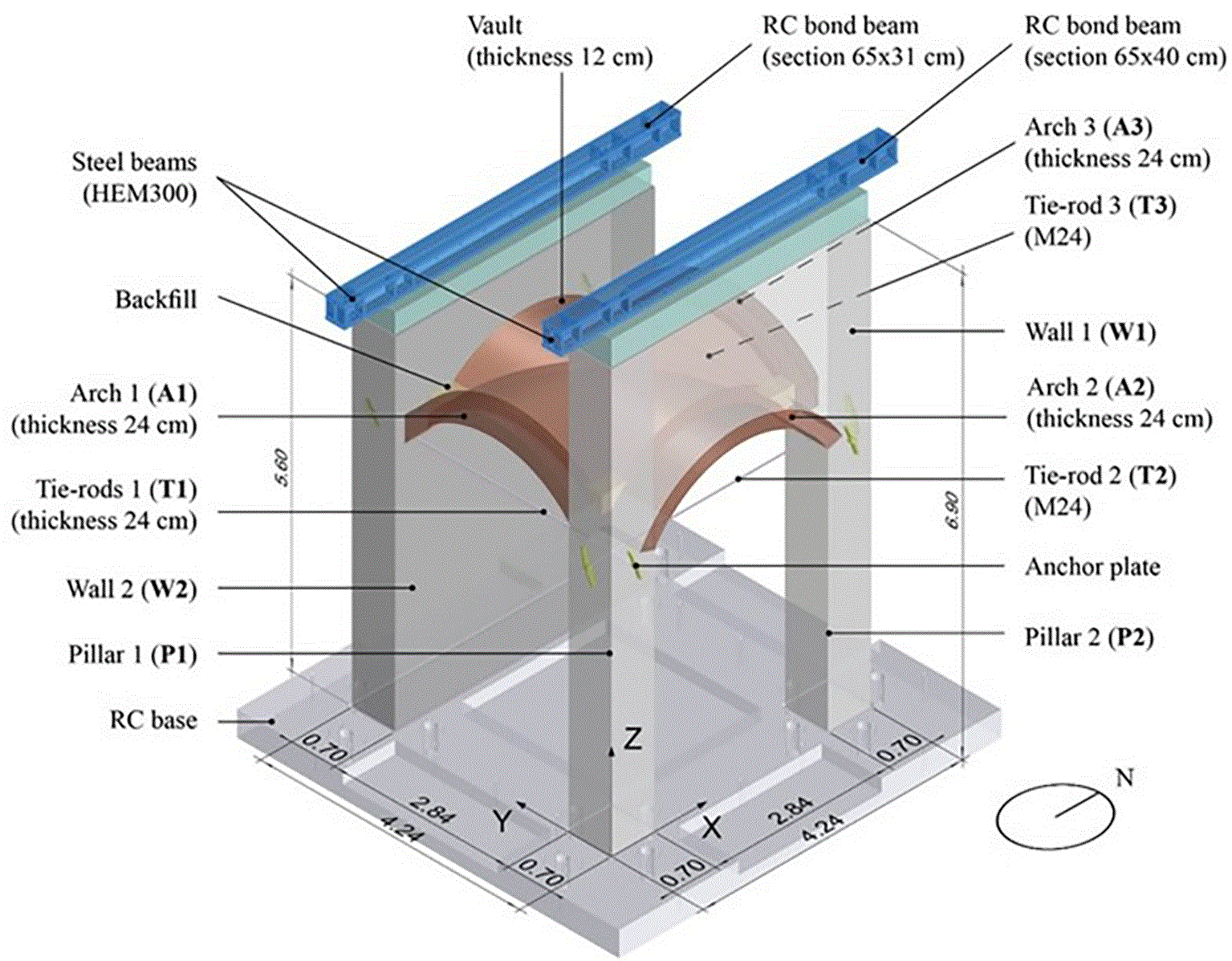
Figure 1. 3D view of the full-scale specimen (dimensions in m).
The construction phase lasted approximately two months, starting in early June 2025 and concluding in early August 2025. The specimen is built upon a reinforced concrete foundation, with a layer of mortar placed between the foundation and the base of the pillars (Pillar 1 and Pillar 2) and of the external wall (Wall 2). The brick masonry cross vault, located at a height of approximately 4 m above the foundation, is bounded on three sides by the arches, two transverse (Arch 1 and Arch 3) and one longitudinal (Arch 2), while the fourth side is bounded by the external wall (Wall 2). Structurally, the vault is supported by both the pillars of the internal wall (Wall 1) and the external wall (Wall 2). At its corners, the vault is toothed into these supporting elements, establishing a mechanical interlocking. The connections between the vault and the arches vary along the perimeter of the vault. In fact, a continuous structural connection exists between the vault and the transverse arches (Arch 1 and Arch 3) along their entire length, while the connection between the vault and both the longitudinal arch (Arch 2) and the external wall (Wall 2) is limited near the springing, introducing a structural discontinuity.
Regarding the materials, the vault and arches are constructed using hand-made solid clay bricks with approximate dimensions of 24 × 12 × 6 cm. The bricks are bonded using a pre-mixed natural hydraulic lime mortar of class M5 (BioCalce Pietra, Kerakoll). The vault is built as a single layer of bricks laid on edge and arranged radially (
Figure 2a). The arches, on the other hand, have a transverse cross-section characterised by the brick arrangement shown in
Figure 2b, in which bricks with their longest side oriented along the radial plane alternate with two superimposed bricks laid on edge.
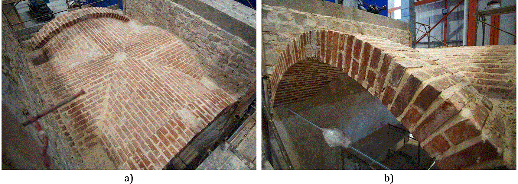
Figure 2. Brick masonry arrangement: a) extrados view, b) brick arrangement of the transverse arches.
At the extrados of the vault, four backfills are constructed at the corners. These consist of stacked brick fragments arranged in multiple layers and bonded with the same mortar used in the brick masonry. Notably, these backfills are not structurally connected to the vault or the adjacent walls.
The vertical walls are built using stone masonry composed of limestone extracted from the Saltrio quarry in the Varese province, Italy.6 The stones are roughly cut, with maximum dimensions ranging from 25–30 cm along the longest side and 15–20 cm along the other sides. They are bonded with the same mortar used for the bricks, enriched with quartz filler, to reduce its compressive strength, and with gravel (4-6 mm). The wall cross-sections are characterised by larger stones placed on the perimeter and smaller stones filling the inner core. The external arrangement of the stones is illustrated in
Figure 3.
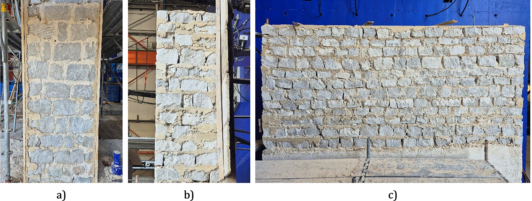
Figure 3. Stone masonry arrangement: a) transverse face of the pillar, b) transverse face of the wall (Wall 2), c) external face of the wall (Wall 2).
Some parts of the specimen, highlighted in orange in
Figure 4, are plastered. The intrados of the vault is plastered with a 5 mm thick mineral-based finishing plaster, while the stone masonry surfaces are plastered with an inner layer made of the same pre-mixed natural hydraulic lime used for the mortar, with the addition of gravel, and finished with the mineral-based finishing plaster. The plaster layers for stone masonry are approximately 10–15 mm thick.
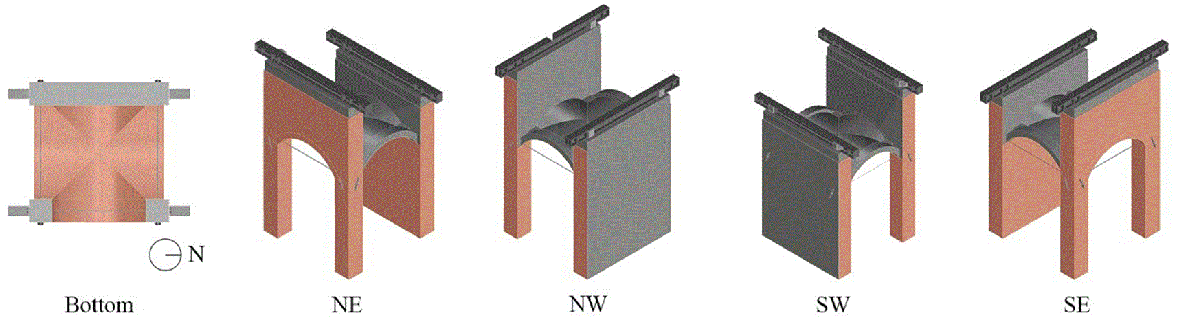
Figure 4. Scheme of the plastered surfaces (in orange).
A system of steel tie-rods, consisting of M24 threaded rods connected to the stone masonry walls metallic anchor plates, are placed just below the springing level of the arches. All the rods and the anchor plates are made of modern steel.
Finally, at the top of both walls (Wall 1 and Wall 2), a reinforced concrete bond beam made of low-strength concrete is placed, together with a steel beam (HEM300) required to attach the actuators to the specimen. The interface between the masonry and the bond beam is intentionally enhanced by leaving the course of stones partially unfilled with mortar, thereby allowing the concrete to penetrate and create a mechanical interlock. Steel connectors are then used to link the concrete bond beams to the overlying steel beams.
Figure 5 shows the specimen after the construction.
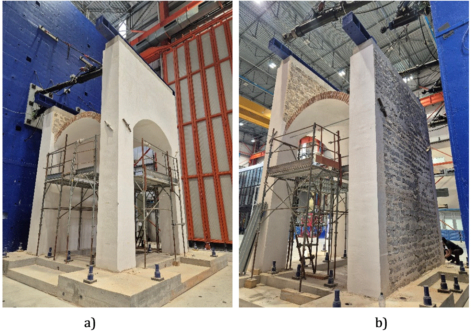
Figure 5. Photograph of the specimen after construction: a) south-east view; b) north-west view.
Strengthened specimen
The structural strengthening intervention, carried out after the first set of PsD tests, was carried out in mid-January 2026. The works involved both the intrados and extrados surfaces of the cross vault and consisted of the installation of a Steel-Reinforced Grout (SRG) system, provided by Kerakoll. In particular, the system used is composed of a unidirectional fibre sheet, made of steel micro-cords and fixed to a fibreglass micromesh (Geosteel G600) combined with a M15 geo-mortar (GeoCalce F Antisismico).
The intervention was performed first treating the existing cracks in the cross vault by mechanically opening and subsequently sealing them at the intrados using the geo-mortar. Subsequently, a fluid grout prepared with the same mortar was poured from the extrados to ensure complete filling of the openings and to restore the continuity of the masonry.
After this first phase, the SRG strengthening system was applied to the extrados according to the scheme shown in
Figure 6. The system consisted of an initial layer of mortar, with a thickness of approximately 3–5 mm, onto which the fibre sheet reinforcement was placed while the mortar was still fresh. The reinforcement was then covered with a second mortar layer with a thickness of approximately 3–5 mm to protect the fibre sheets.
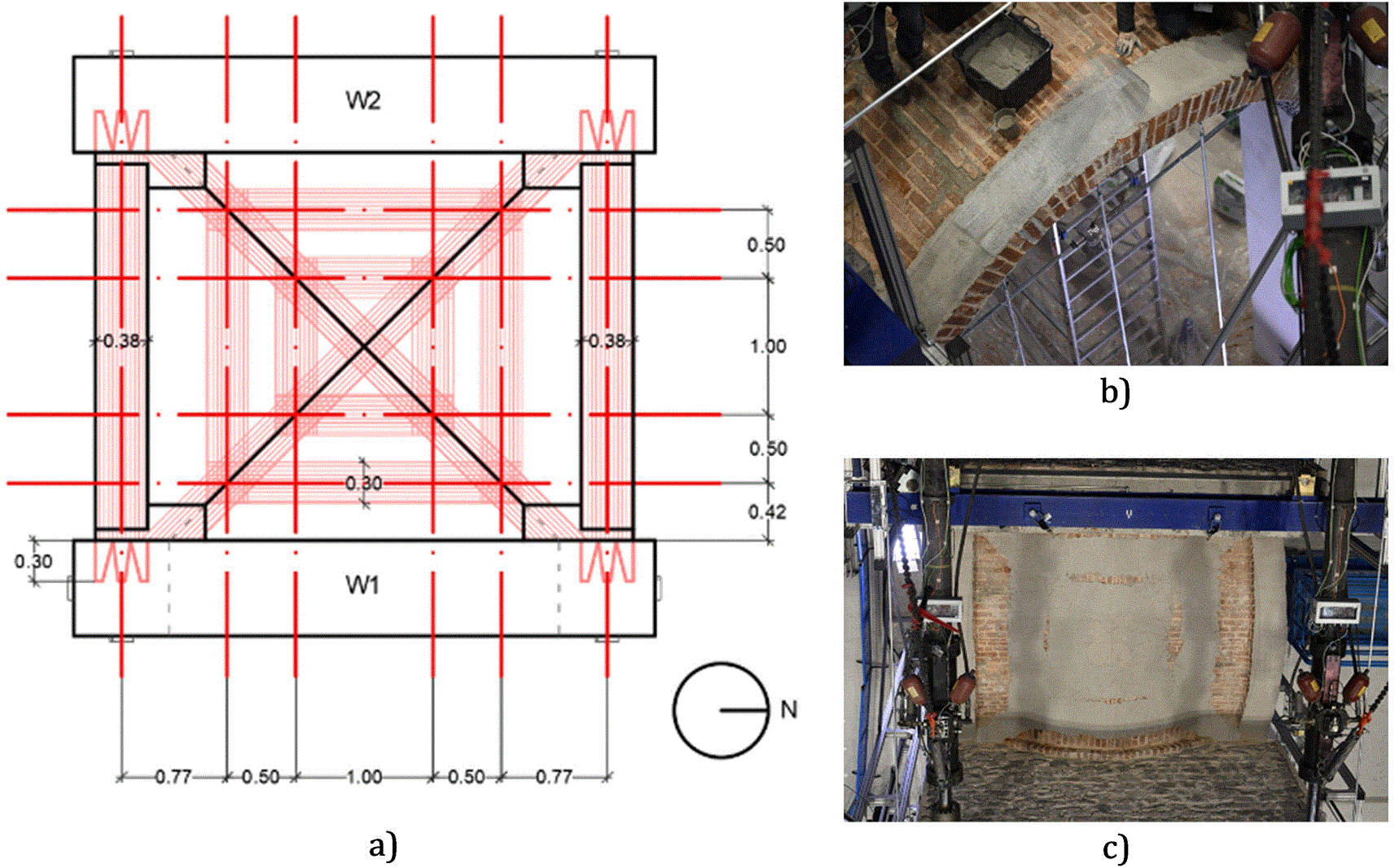
Figure 6. a) Application scheme of the SRG system at the extrados (dimensions in m); b) photograph of the application of the fibre sheet at the extrados of the transverse arch; c) photograph of the completed strengthening intervention.
The fibre sheets applied along the transverse arches were mechanically anchored to the adjacent walls by drilling three holes into the masonry and inserting the cut ends of the sheets into the holes for an anchorage length of approximately 30 cm.
Material properties
To characterise the mechanical properties of the materials employed in the construction of the specimen, both destructive and non-destructive tests were conducted on masonry units as well as on assembled masonry. These properties are essential for the interpretation of the experimental results and for the calibration of the numerical models. In this section, only the main results are briefly reported and they are summarised in
Table 1.
Table 1. Results of destructive and non-destructive tests carried out on stone and brick units.
| Material | Test type | No. of specimens | Mean value(s) | Standard(s) |
|---|
| Saltrio stone | Apparent density, open porosity | 6 | ρβ ≈ 2690 kg/m3; ρo ≈ 0.4 | EN 1936:2006 |
| Dynamic modulus (UPV) | 19 (⊥ and//) | Ed ≈ 63-70 GPa (direction-dependent) | |
| Static modulus in compression | 19 | Es ≈ 62-71 GPa | EN 12390-1, -2 |
| Compressive strength | 19 | fc ≈ 114-157 MPa (orientation-dependent) | EN 12390-1, -2 |
| Flexural tensile strength | – | ftc,f ≈ 18.6 MPa | EN 12372:2022 |
| Splitting tensile (Brazilian) | – | ftc,B ≈ 6.46 MPa | EN 12390-6 (by analogy) |
| Clay bricks | Flexural tensile strength | 11 | ft ≈ 6.18 MPa | EN 772-1 |
| Compressive strength | 22 | fc ≈ 15.8 MPa | EN 772-1 |
| Physical properties | – | ρ ≈ 1620 kg/m3; size 6 × 12 × 24 cm | |
The properties of the Saltrio stone are taken from the literature,6 while brick properties are derived from experimental tests. The results show that Saltrio stone exhibits high stiffness and strength, with both dynamic and static elastic moduli in the range of 60–70 GPa and compressive strength exceeding 100 MPa. The clay bricks show significantly lower strength, with compressive strength around 16 MPa.
Sonic tests were conducted at the masonry level, on the external stone wall (Wall 2), on stone pillars (Pillar 1 and Pillar 2) and on the brick vault and arches to derive in-situ
estimates of the dynamic Young’s modulus of masonry.
Both direct and indirect sonic test configurations were adopted, with multiple measurement paths along the height and span of the elements. The measured pulse velocities, combined with assumptions on material density, were used to back-calculate dynamic moduli. The results are summarised in
Table 2.
Table 2. Dynamic Young’s modulus of stone and brick masonry derived from sonic test results.
| Structural Element | Materials | n (pairs × velocities) * | Test type | Dynamic Young’s Modulus [GPa] |
|---|
| min-max
| AVG | COV |
|---|
| Wall 2 | Stone | 4 × 20 | Direct tests | 5.8 – 13.6 | 9.6 | 36% |
| Pillar 1/Pillar 2 | Stone | 2 × 20 | Direct tests | 9.0-12.9 | 9.9 | 26% |
| 2 × 20 | Indirect tests | 10.4-18.7 | 13.7 | 34% |
| Vault and Arch 3 | Brick | 2 × 20 | Direct tests | 2.6-4.4 | 3.5 | 36% |
| 2 × 20 | Indirect tests | 2.6 – 5.1 | 3.9 | 44% |
Dynamic identification tests
Dynamic identification tests were performed on the as-built and strengthened configurations through ambient vibration tests under laboratory conditions. It is worth recalling that the previously mentioned reinforced concrete and steel beams were present at the top of the two walls during the dynamic identification tests. The setup included piezoelectric accelerometers (10 V/g sensitivity) and a data acquisition system with a sampling frequency of 200 Hz. During testing, the specimen was simply supported at the base and free at the top. The experimental data were postprocessed using Artemis Modal.
For the as-built configuration, the accelerometer layout is shown in
Figure 7, and nine relevant modes were identified in the frequency range between 4.98 Hz and 93.07 Hz (
Figure 8).
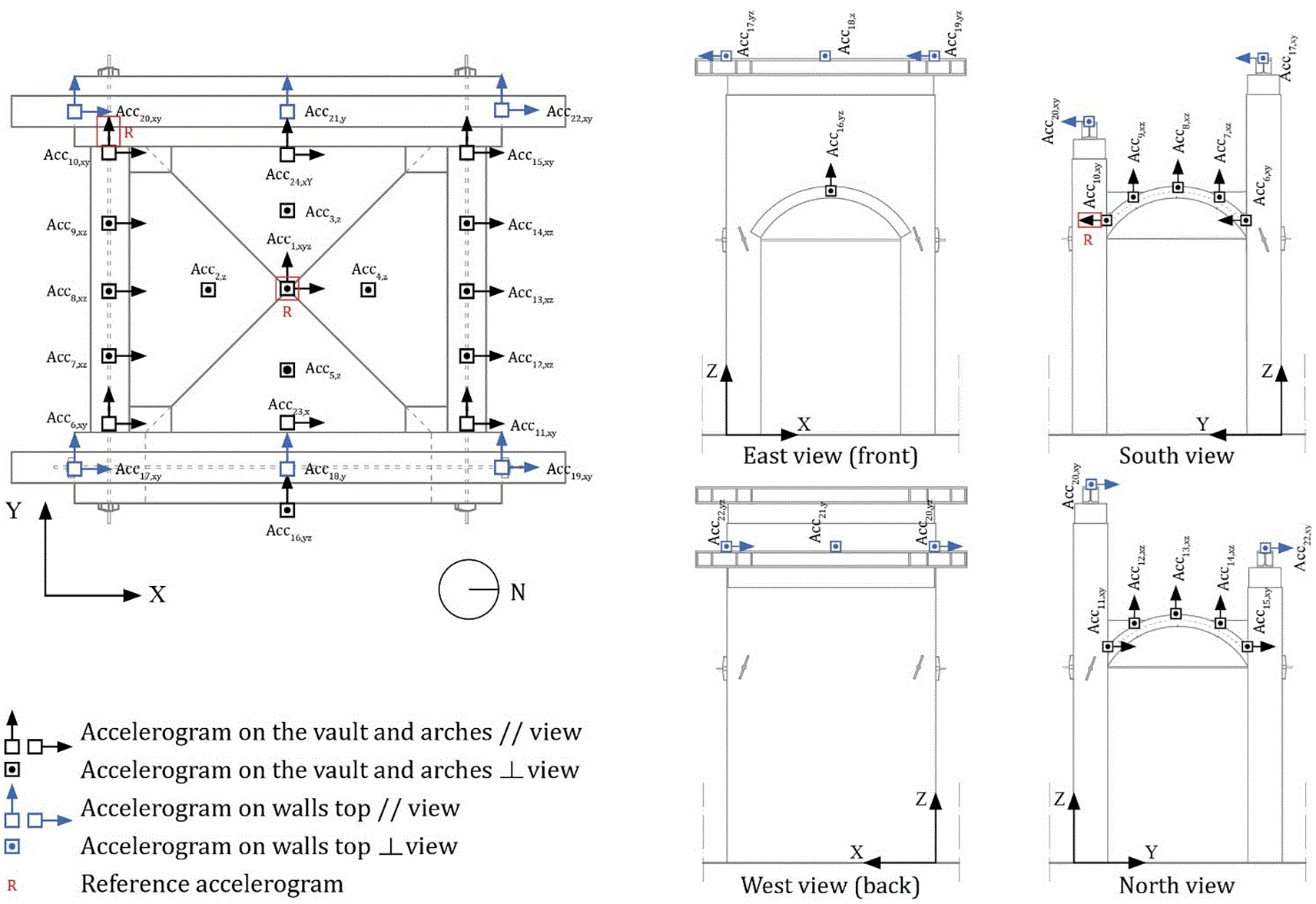
Figure 7. Instrumentation layout and accelerometer positions.
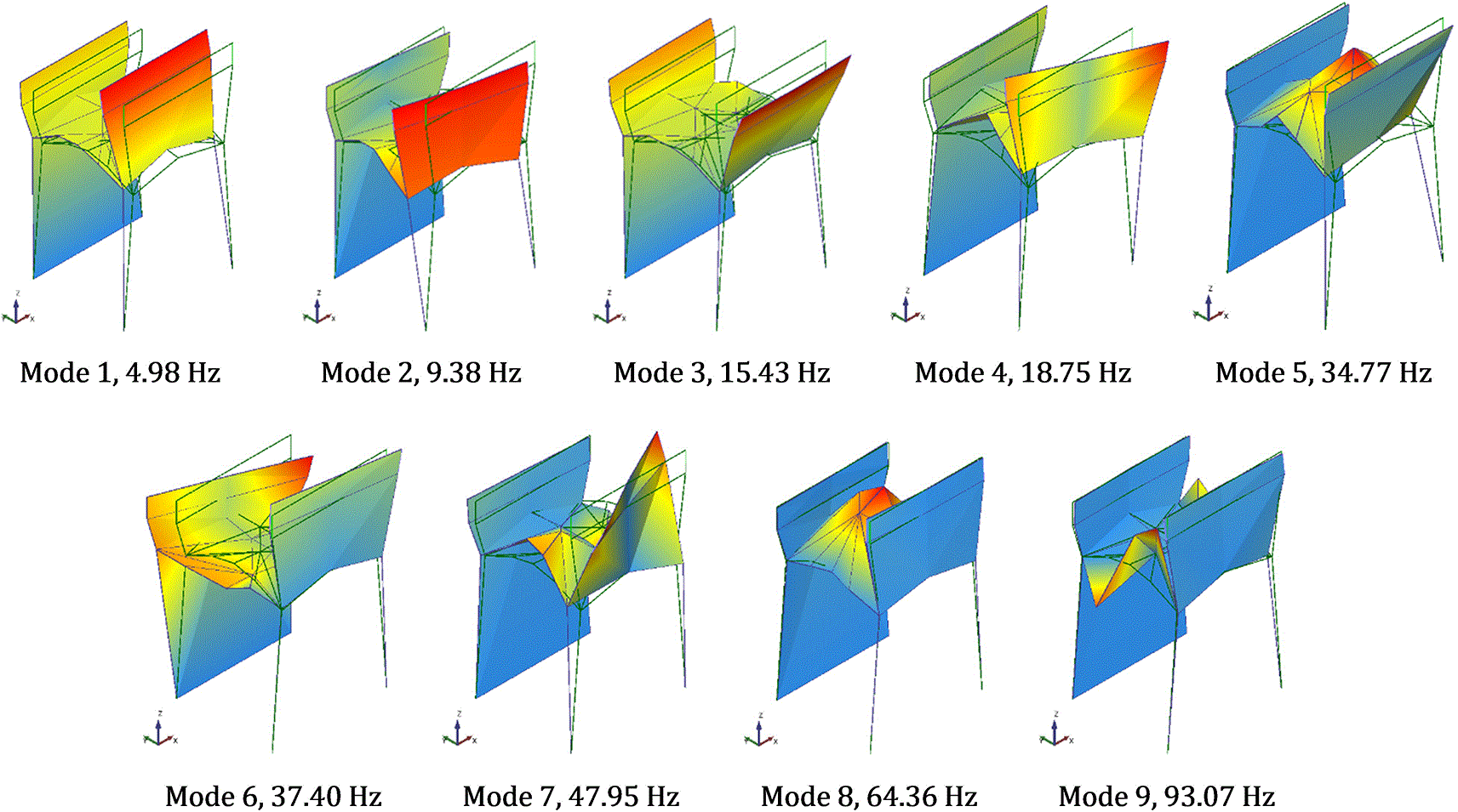
Figure 8. Identified vibration modes of the as-built configuration of the specimen from dynamic identification tests.
For the dynamic identification tests performed on the strengthened configuration, the same boundary conditions were maintained (simply supported at the base and free at the top), and ambient vibration tests were carried out under the same laboratory conditions. The accelerometers were positioned in the same locations of the as-built configuration (
Figure 7). In this case, eight modes were identified within the frequency range of 4.40–58.69 Hz (
Figure 9). Based on the analysis of the mode shapes and the comparison of the MAC values between the as-built and strengthened configurations, the modal sequence remains unchanged, with the exception of modes 5 and 6, which appear inverted in the strengthened configuration. In addition, a general decrease in frequencies is observed, and mode 9 could not be identified in the strengthened configuration. A detailed discussion of the comparison between the as-built and the strengthened configuration is beyond the scope of the present work and is therefore not addressed here.
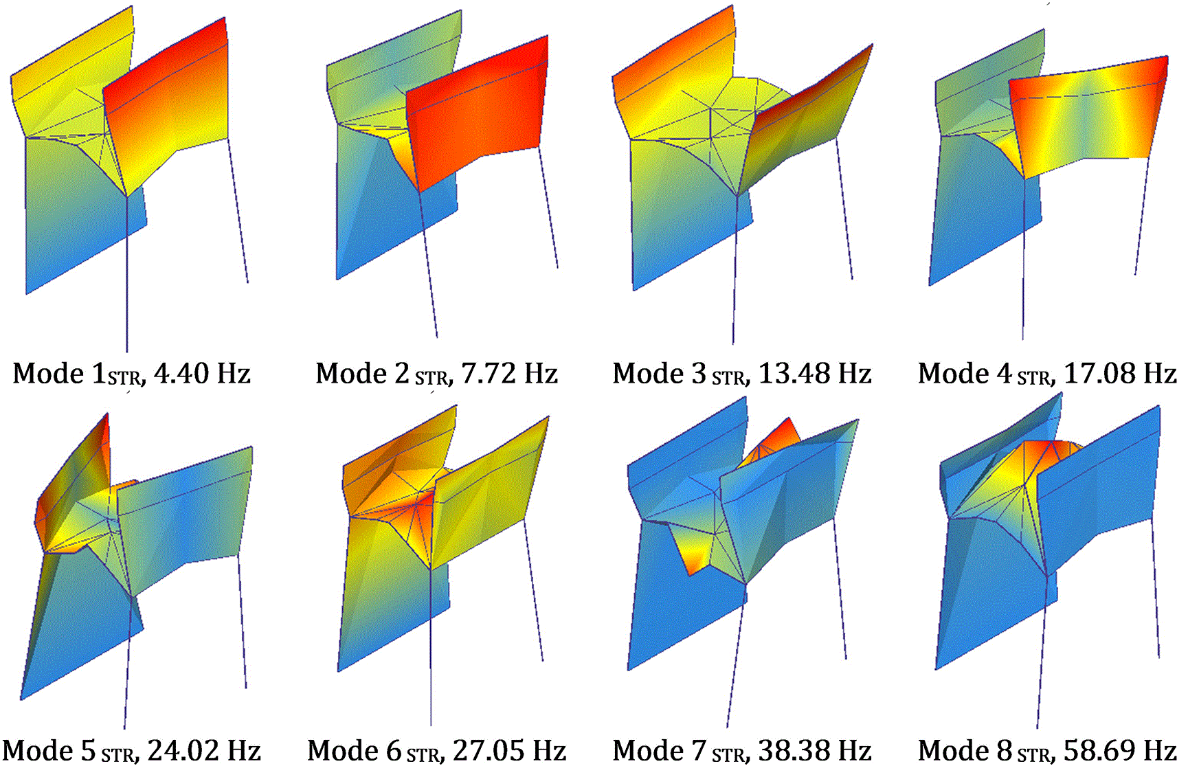
Figure 9. Identified vibration modes of the strengthened configuration of the specimen from dynamic identification tests.
The experimental campaign
The experimental campaign aimed at evaluating both the response of the as-built structure and the effectiveness of the strengthening intervention based on Steel Reinforced Grout (SRG) technique, by structuring the campaign in two main phases. In the first phase, the specimen was tested in its as-built configuration, while in the second phase, after the application of the SRG strengthening system, the specimen was re-tested under the same loading conditions.
The experimental investigation was conducted under displacement-controlled conditions, with two independent horizontal longitudinal Degrees of Freedom, DoF1 and DoF2, applied at the top of the walls (
Figure 10). This configuration was selected to reproduce the differential seismic displacements of the two walls, thus activating the in-plane shear mechanisms in the cross vault.
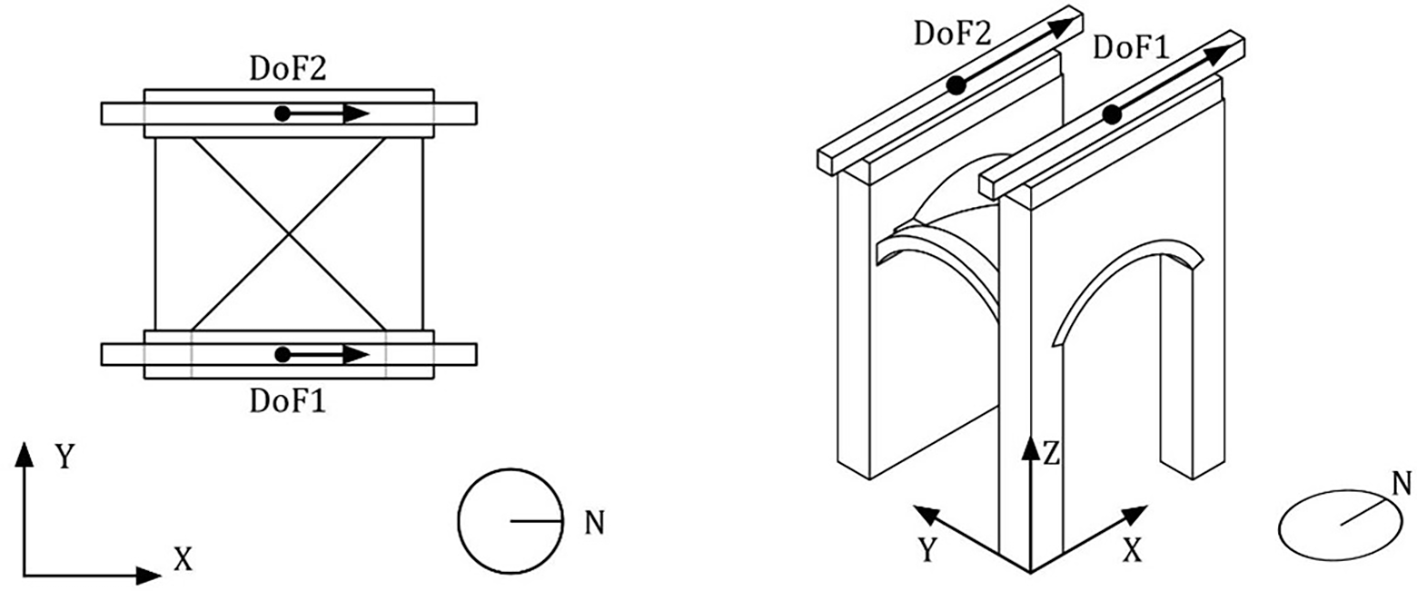
Figure 10. Location of DoF1 and DoF2 selected for the PsD test.
The following sections provide a detailed description of the actuator configuration, control strategy, instrumentation layout, and loading protocol.
Set-up and instrumentation
This section describes the actuators employed in the experimental setup, including their functional roles and technical specifications, as well as the instrumentation used to monitor displacements and forces during testing.
Schematic views of the test set-up, the orientation of the specimen (having the reaction wall on the west side), and the labels of the structural elements are presented in
Figure 11. All the actuators were attached to the rigid steel beams bolted at the top of two stone masonry walls (i.e. Wall 1 and Wall 2 on the east and west side, respectively). Each interface beam connected five actuators used to apply both the vertical permanent load (counteracted by the foundation) and the horizontal seismic action (counteracted by the lab strong-wall), as well as to apply the selected boundary conditions. In more detail, for every wall:
- 3 actuators laying in the horizontal plane controlled the horizontal co-ordinates, longitudinal south-to-north (X) translation, transversal east-to-west (Y) translation and rotation about the vertical axis (RZ);
- 2 actuators mounted vertically at the north and south ends of the beam controlled the vertical load and the rotation around the Y axis (for Wall 1) or the vertical load and the moment around the Y axis (for Wall 2).
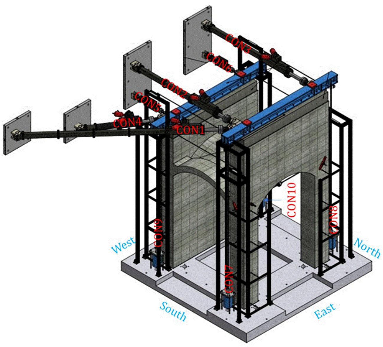
Figure 11. Schematic view of the specimen, including orientation, actuators label.
Next
Table 3 gathers the main characteristics of the 10 installed actuators, while
Table 4 lists the variables of the actuator co-ordinate system and
Table 5 the ones relative to the modal-control co-ordinate system.
Table 5 also includes the actuators involved in the control of each DoF and the variable chosen for the control. The labels adopted to identify each variable are set according to the nomenclature reported in the following:
Table 3. Characteristics of actuators installed on the specimen.
| Label | Total stroke [mm] | Maximum force [kN] |
Position |
|---|
| CON 1 | 1000 | ± 500 | Wall 1 horizontal |
| CON 2 | 1000 | ± 500 | Wall 1 horizontal |
| CON 3 | 1000 | ± 500 | Wall 1 horizontal |
| CON 4 | 500 | ± 500 | Wall 2 horizontal |
| CON 5 | 250 | ± 190 | Wall 2 horizontal |
| CON 6 | 250 | ± 190 | Wall 2 horizontal |
| CON 7 | 230 | ± 780 (
*) | Wall 1 vertical |
| CON 8 | 230 | ± 780 (
*) | Wall 1 vertical |
| CON 9 | 230 | ± 780 (
*) | Wall 2 vertical |
| CON 10 | 230 | ± 780 (
*) | Wall 2 vertical |
Table 4. Piston co-ordinate system.
| Piston co-ordinate | Displacement quantity | Force quantity | Direction | Position |
|---|
| CON1 |
|
| Pulling along the actuator axis | Wall 1 horizontal |
| CON2 |
|
| Pulling along the actuator axis | Wall 1 horizontal |
| CON3 |
|
| Pulling along the actuator axis | Wall 1 horizontal |
| CON4 |
|
| Pulling along the actuator axis | Wall 2 horizontal |
| CON5 |
|
| Pulling along the actuator axis | Wall 2 horizontal |
| CON6 |
|
| Pulling along the actuator axis | Wall 2 horizontal |
| CON7 |
|
| Pulling along the actuator axis | Wall 1 vertical |
| CON8 |
|
| Pulling along the actuator axis | Wall 1 vertical |
| CON9 |
|
| Pulling along the actuator axis | Wall 2 vertical |
| CON10 |
|
| Pulling along the actuator axis | Wall 2 vertical |
Table 5. Modal-control co-ordinate system.
| Mode | Displacement (rotation) quantity | Force quantity | Direction | Position |
Involved actuators | Controlled variable | PsD DoF or Boundary Condition (BC) |
|---|
| 1 |
|
| X | Wall 1 horizontal | CON1, CON2, CON3 |
| PsD DoF1 |
| 2 |
|
| Y | Wall 1 horizontal | CON1, CON2, CON3 |
| BC: set constant equal to 0 |
| 3 |
|
| Z (Ɵ) | Wall 1 horizontal | CON1, CON2, CON3 |
| BC: set constant equal to 0 |
| 4 |
|
| X | Wall 2 horizontal | CON4, CON5, CON6 |
| PsD DoF2 |
| 5 |
|
| Y | Wall 2 horizontal | CON4, CON5, CON6 |
| BC: set constant equal to 0 |
| 6 |
|
| Z (Ɵ) | Wall 2 horizontal | CON4, CON5, CON6 |
| BC: set constant equal to 0 |
| 7 |
|
| -Z | Wall 1 vertical | CON7, CON8 |
| BC: set constant equal to 200 kN |
| 8 |
|
| -Y (-β) | Wall 1 vertical | CON7, CON8 |
| BC: set constant equal to 0 |
| 9 |
|
| -Z | Wall 2 vertical | CON9, CON10 |
| BC: set constant equal to 20 kN |
| 10 |
|
| -Y (-β) | Wall 2 vertical | CON9, CON10 |
| BC: set constant equal to 0 |
For the sake of clarity, two examples are given:
is the control-mode rotational displacement (i.e. rotation about Z axis) at the top of Wall 1;
is the control-mode force along Z axis at the top of Wall 2 (i.e. compression on Wall 2).
During the experiments the specimen was monitored by several instruments. Each actuator includes an embedded displacement sensor (Temposonics) and a load cell, measuring the displacement and applied load in the direction of the actuators. Clearly, such quantities need to be combined to obtain the corresponding quantities in the XYZ reference system, in which the control-mode quantities are considered. Additionally, ten displacement sensors (optical linear encoders, Heidenhain MSA 375) connected to a reference frame were monitoring the motion of the specimen at the actuators location along the XYZ reference system. Practically speaking, these instruments were mounted parallel to the actuators, with the exception of CON1 and CON4; for these last two, the sensors were mounted along the X axis, hence directly measuring
and
displacements. All of these displacement and force sensors follow the numbering of the actuators.
During the tests, the movements of the specimen were also monitored using potentiometer displacement transducers (Gefran 50 mm and 100 mm) placed close to the four corners of the specimen along both X and Y directions. Additionally, three potentiometers on both the north and south arches were recording their vertical motions. Finally, the tensile force applied by the arches’ ties was monitored by load cells (HBM) mounted at mid-length. Next
Figure 12 schematically shows the position of the sensors mounted on the specimen, while gathers the complete list of sensors summarising their labels, types, ranges, monitored element, monitored side or direction, and mounting position. Note that the labels of the instruments include most of the information shown by
Table 6 being, in most cases, formed by joining:
- the type of instrument (potentiometer POT or load cell LC);
- the monitored element (named according to
Figure 12, e.g. P1, W2N, A1, etc.);
- the monitored side (i.e. N, S, E, W) only for the vertical elements;
- the mounting position along the length of the element:
o height for the vertical elements in thirds (i.e. 0 to 3);
o the side for the arches (i.e. west W, middle M or east E), the sensors are mounted at the quarters of the length of the elements.
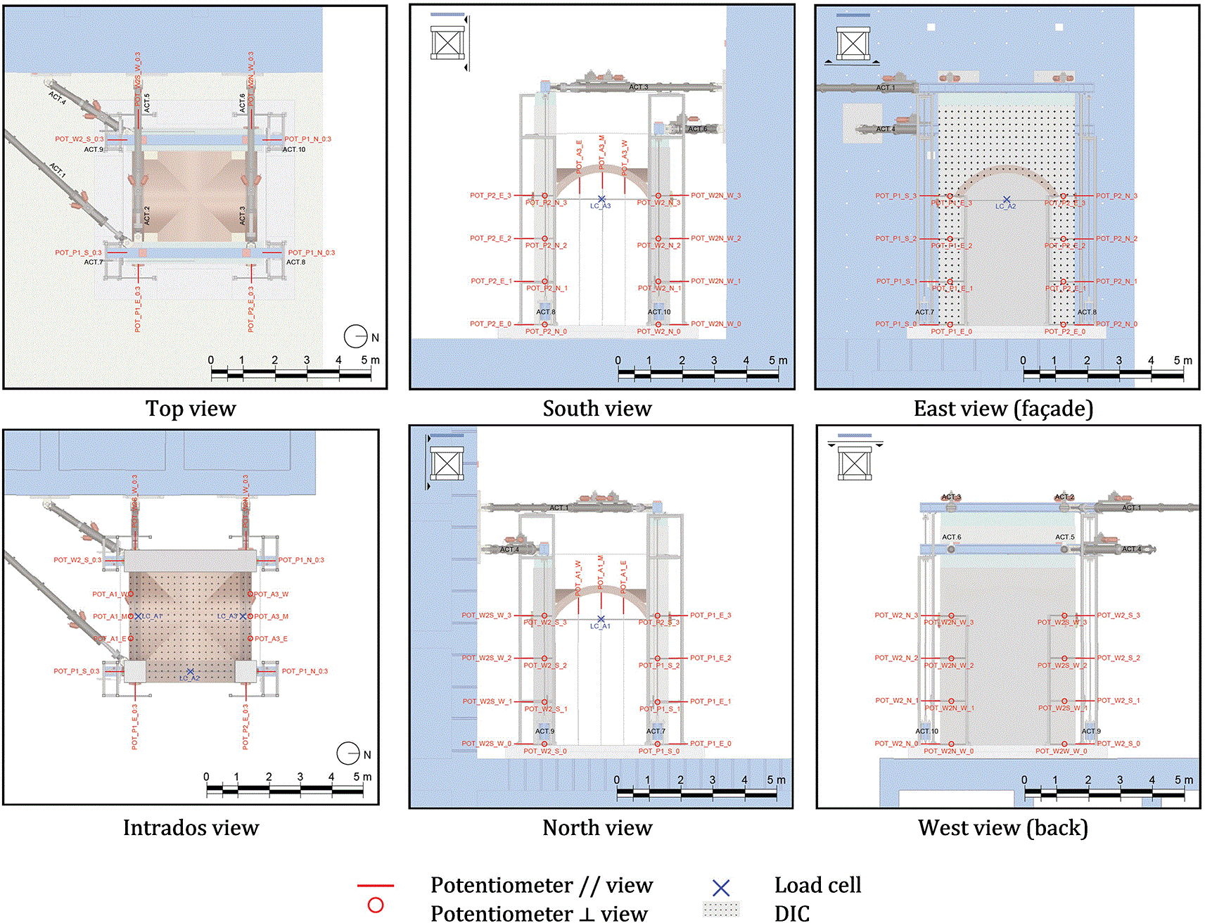
Figure 12. Schematic view position of installed instruments.
Table 6. List of sensors installed on the specimen.
| Label | Type | Range | Element | Side/Direction | Mounting position |
|---|
| POT_P1_S_0
| Potentiometer | 50 mm | Pillar P1 | South/X | 0 (Base) |
| POT_P1_S_1
| Potentiometer | 100 mm | Pillar P1 | South/X | 1/3 of height |
| POT_P1_S_2
| Potentiometer | 100 mm | Pillar P1 | South/X | 2/3 of height |
| POT_P1_S_3
| Potentiometer | 100 mm | Pillar P1 | South/X | 3/3 of height |
| POT_P1_E_0
| Potentiometer | 50 mm | Pillar P1 | East/Y | 0 (Base) |
| POT_P1_E_1
| Potentiometer | 100 mm | Pillar P1 | East/Y | 1/3 of height |
| POT_P1_E_2
| Potentiometer | 100 mm | Pillar P1 | East/Y | 2/3 of height |
| POT_P1_E_3
| Potentiometer | 100 mm | Pillar P1 | East/Y | 3/3 of height |
| POT_P2_N_0
| Potentiometer | 50 mm | Pillar P2 | North/X | 0 (Base) |
| POT_P2_N_1
| Potentiometer | 100 mm | Pillar P2 | North/X | 1/3 of height |
| POT_P2_N_2
| Potentiometer | 100 mm | Pillar P2 | North/X | 2/3 of height |
| POT_P2_N_3
| Potentiometer | 100 mm | Pillar P2 | North/X | 3/3 of height |
| POT_P2_E_0
| Potentiometer | 50 mm | Pillar P2 | East/Y | 0 (Base) |
| POT_P2_E_1
| Potentiometer | 100 mm | Pillar P2 | East/Y | 1/3 of height |
| POT_P2_E_2
| Potentiometer | 100 mm | Pillar P2 | East/Y | 2/3 of height |
| POT_P2_E_3
| Potentiometer | 100 mm | Pillar P2 | East/Y | 3/3 of height |
| LC_A1 | Load cell | ±125 kN | Tie on arch A1 | - /Axial | Middle |
| LC_A2 | Load cell | ±125 kN | Tie on arch A2 | - /Axial | Middle |
| LC_A3 | Load cell | ±125 kN | Tie on arch A3 | - /Axial | Middle |
| POT_W2N_N_0
| Potentiometer | 50 mm | Wall 2 North end W2N | North/X | 0 (Base) |
| POT_W2N_N_1
| Potentiometer | 50 mm | Wall 2 North end W2N | North/X | 1/3 of height |
| POT_W2N_N_2
| Potentiometer | 50 mm | Wall 2 North end W2N | North/X | 2/3 of height |
| POT_W2N_N_3
| Potentiometer | 50 mm | Wall 2 North end W2N | North/X | 3/3 of height |
| POT_W2N_W_0
| Potentiometer | 50 mm | Wall 2 North end W2N | West/Y | 0 (Base) |
| POT_W2N_W_1
| Potentiometer | 50 mm | Wall 2 North end W2N | West/Y | 1/3 of height |
| POT_W2N_W_2
| Potentiometer | 50 mm | Wall 2 North end W2N | West/Y | 2/3 of height |
| POT_W2N_W_3
| Potentiometer | 50 mm | Wall 2 North end W2N | West/Y | 3/3 of height |
| POT_A3_W
| Potentiometer | 50 mm | North arch A3 | Intrados/Z | West quarter |
| POT_A3_M
| Potentiometer | 50 mm | North arch A3 | Intrados/Z | Middle |
| POT_A3_E
| Potentiometer | 50 mm | North arch A3 | Intrados/Z | East quarter |
| POT_W2S_S_0
| Potentiometer | 50 mm | Wall 2 South end W2S | South/X | 0 (Base) |
| POT_W2S_S_1
| Potentiometer | 50 mm | Wall 2 South end W2S | South/X | 1/3 of height |
| POT_W2S_S_2
| Potentiometer | 50 mm | Wall 2 South end W2S | South/X | 2/3 of height |
| POT_W2S_S_3
| Potentiometer | 50 mm | Wall 2 South end W2S | South/X | 3/3 of height |
| POT_W2S_W_0
| Potentiometer | 50 mm | Wall 2 South end W2S | West/Y | 0 (Base) |
| POT_W2S_W_1
| Potentiometer | 50 mm | Wall 2 South end W2S | West/Y | 1/3 of height |
| POT_W2S_W_2
| Potentiometer | 50 mm | Wall 2 South end W2S | West/Y | 2/3 of height |
| POT_W2S_W_3
| Potentiometer | 50 mm | Wall 2 South end W2S | West/Y | 3/3 of height |
| POT_A1_W
| Potentiometer | 50 mm | South arch A1 | Intrados/Z | West quarter |
| POT_A1_M
| Potentiometer | 50 mm | South arch A1 | Intrados/Z | Middle |
| POT_A1_E
| Potentiometer | 50 mm | South arch A1 | Intrados/Z | East quarter |
For the sake of clarity and simplicity of understanding, a few examples are given in the following:
-
POT_P1_S_1: potentiometer monitoring pillar P1, mounted on the south side at 1/3 of the height of the element;
- LC_A1: load cell monitoring the tie of south arch A1;
-
POT_W2N_W_2: potentiometer monitoring the north end of Wall 2, mounted on the north side at 2/3 of the height of the element;
-
POT_A3_W: potentiometer monitoring the north arch A3, mounted on the west side (at 1/4 of its length).
Please note that the calibration reports of all force and displacement sensors are included in the dataset. For additional details about the interpretation of the calibration reports, the reader can refer to the Technical Report No JRC139347.7
During the tests, ELSAREC, the ELSA REal-time Controller (for further details, refer to8), was used to monitor the response of the whole testing setup running multiple acquisitions in parallel. This includes signals of the standard instruments (i.e. potentiometers and load cells) as well as signals from the control system (e.g., actuator and control variables). Some continuous acquisitions were running at 10 Hz, while some others (record average) were sampled at a variable rate. These last acquisitions recorded the average values available at the conclusion of each step (record) of the loading pattern. During the pseudo-dynamic tests, for the variables involved in the equation of motion, only the record average acquisition is available. It has to be noted that the prototype-time variable, common to both acquisition files, can be used for synchronisation purposes. For further detail, refer to the Technical Report No JRC141264.9
Besides all the instruments mentioned above, the east side of the specimen and the intrados of the vault were monitored using stereo Digital Image Correlation (DIC). For the east façade, two digital cameras controlled and synchronised by ELSAREC, acquired high resolution photographs at regular time intervals. For the intrados, four digital cameras (organised in two independent stereo camera sets) were positioned at ground level on vault edges to monitor the northern and southern sections of the vault footprint. This allowed the recording of the whole intrados at a regular frequency of 0.25 Hz during the whole test campaign. By cross-correlating images between cameras and through time, this contactless measuring technique is able to reconstruct 3D dimensional geometry of the vault and its displacement fields. This allows tracking the formation and propagation of cracks during the experiment.
Figure 13 shows the south-east side of the specimen with the random speckle patterns used by the DIC technique to track displacements. Note that the DIC images will be stored in a separate public dataset that will be published in the near future (when available, the link to this second dataset gathering DIC images only will be added on the ERIES-REVAULTs dataset object of this paper).
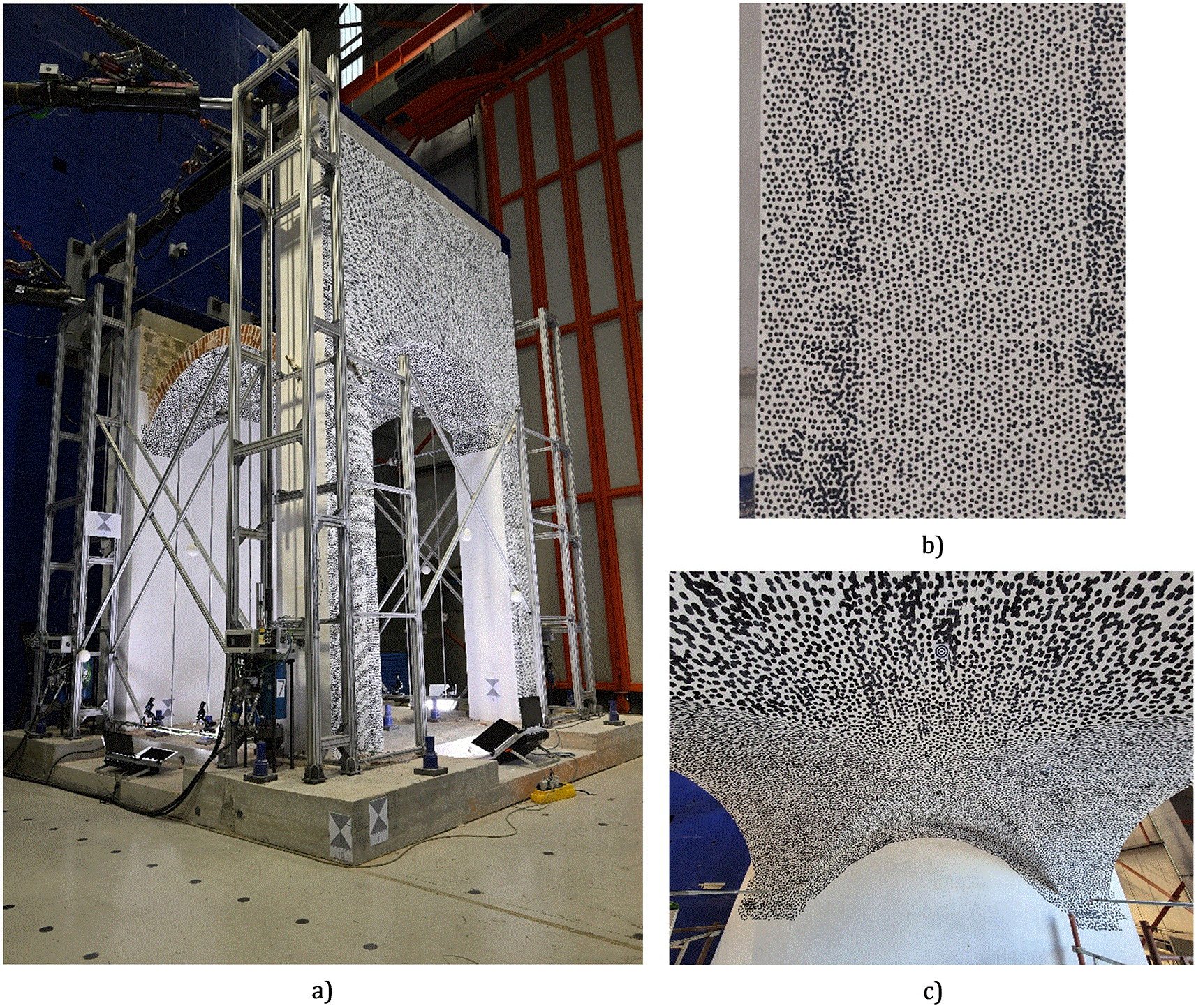
Figure 13. View of the specimen (a) and the random speckle pattern applied for DIC: b) east façade; c) intrados.
Test programme and loading input
As mentioned in the previous sections, the experimental campaign involved two testing phases: first, the specimen was tested in its as-built configuration, then it was repaired and reinforced using steel fibres reinforced grout, and finally it was retested in the retrofitted configuration.
The shared data belong to both phases, each of them includes a preliminary pseudo-static test, useful for the determination of the initial stiffness, and several Pseudo-Dynamic (PsD) hybrid experiments at increasing amplitude.
Table 7 summarises the complete list of experiments origin of the data included in the dataset.
Table 7. List of performed experiments.
| Experiment tag | Description | Maximum amplitude | Specimen configuration |
|---|
| c01 | Cyclic (determination of stiffness) | 1 mm | As-built
|
| c05 | Pseudo-Dynamic
| 10% | As-built
|
| c06 | Pseudo-Dynamic
| 25% | As-built
|
| c07 | Pseudo-Dynamic
| 75% | As-built
|
| c08 | Pseudo-Dynamic
| 100% | As-built
|
| c09 | Pseudo-Dynamic
| 125% | As-built
|
| c10 | Pseudo-Dynamic
| 150% | As-built
|
| d02 | Cyclic (determination of stiffness) | 1 mm | Retrofitted |
| e01 | Pseudo-Dynamic
| 25% | Retrofitted |
| e02 | Pseudo-Dynamic
| 75% | Retrofitted |
| e03 | Pseudo-Dynamic
| 100% | Retrofitted |
| e04 | Pseudo-Dynamic
| 125% | Retrofitted |
| e06 | Pseudo-Dynamic
| 150% | Retrofitted |
The input accelerogram was introduced in the X direction for the PsD tests and was derived from the ground motion record of L’Aquila earthquake (6th of April 2009 – AQA; L’Aquila – v. Aterno – F. Aterno). The original accelerogram duration was cropped from 25 s to approximately 10 s, to limit the overall test duration.
Figure 14 shows the input accelerogram adopted as input for the PsD tests, also including the zero padding on the last 0.5 s included to set the specimen in free vibration. The original sampling of the accelerogram was 0.05 s of prototype time, but for the tests it was decided to use a resampled version (through linear interpolation) with a sampling of 0.001 s. Using the continuous PsD method at ELSA, the prototype time input increment (Recording Increment of 0.001 s) is subdivided for the integration in a number of internal time increments (InterRec = 500 in this case) but only the average value of every variable is saved for every Recording Increment.
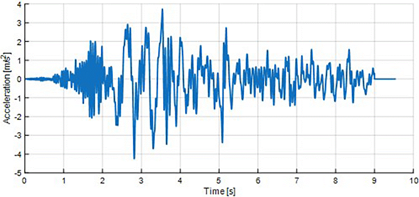
Figure 14. Acceleration time-history input of the PsD tests (100% intensity).
A lumped mass matrix was used for the equation of motion with masses of 21569 and 8071 kg associated, respectively, to the DoFs of Wall1 and Wall 2 in the X direction
Conclusions
This paper presents the dataset generated within the ERIES-REVAULTs experimental campaign, which involved full-scale Pseudo-Dynamic (PsD) testing of a masonry cross-vault system representative of the lateral nave bays of historic masonry churches. The campaign was designed to investigate the in-plane shear response induced by differential longitudinal displacements of the vault supports, a damage mechanism frequently observed in post-earthquake surveys of historical masonry structures.
The shared dataset documents both the as-built and the retrofitted configurations of the specimen, the latter strengthened using a Steel-Reinforced Grout (SRG) system. This work makes available a set of full-scale experimental data on a complex masonry vaulted system tested under hybrid seismic simulation. The dataset is expected to support a wide range of future studies, including the calibration and validation of numerical models, the assessment of strengthening effectiveness, the interpretation of crack development and displacement patterns, and the comparison of alternative seismic assessment and retrofit strategies for masonry historical structures.
Ethic and consent
Ethical approval and consent were not required.
Data availability
Zenodo. REVAULTs: Response Evaluation of masonry VAULTs under pseudo-dynamic loadings: dataset
https://doi.org/10.5281/zenodo.19552030 [10].
This project contains the following underlying data:
REVAULTs_v1.zip. The zip file, once extracted, allows accessing to the whole dataset. The information is accessible to a standard filesystem structure. Due to its complexity, in order to understand the structure of the shared dataset, the reader should refer to the Technical Report No JRC141264.9 A short list of the main contents includes (i) details of the specimens, (ii) applied loading patterns, (iii) details and calibration reports relative to the installed instrumentations (for further details on the calibration procedure, refer to the Technical Report No JRC1393477). Besides, for each test, the dataset includes: (i) raw data as recorded by the acquisition system of the ELSA lab, (ii) processed data for an easier access to the output of the monitoring, (iii) graphical representation of the main response quantities.
The dataset is under embargo until 30/11/2026, as provided for in the grant agreement. Data is available under the terms of the CC BY 4.0 license.
The paper briefly presents the ERIES-REVAULTs project, including all relevant information regarding the specimens, measuring equipment, test setup and test procedure. Future publications will include detailed analyses and discussion of the results. The dataset, gathering quantitative information and metadata, is made available by the authors in line with the requirement of the framework of the ERIES Project [Grant agreement ID: 101058684, https://doi.org/10.3030/101058684]. The complete dataset can be downloaded at https://doi.org/10.5281/zenodo.19552030 under a CC BY 4.0 license.
Acknowledgements
The authors acknowledge the contributions of all team members of the ERIES-REVAULTs project who are not authors of this paper. The authors are also thankful for all the help and support of the staff at the JRC ELSA facility, without whom this experimental campaign could not have been successfully completed.
References
- 1.
Rossi M, Calderini C, Lagomarsino S:
Experimental testing of the seismic in-plane displacement capacity of masonry cross vaults through a scale model.
Bull. Earthq. Eng.
Jan. 2016; 14(1): 261–281. Publisher Full Text
- 2.
Bianchini N, Mendes N, Calderini C, et al.:
Seismic response of a small-scale masonry groin vault: experimental investigation by performing quasi-static and shake table tests.
Bull. Earthq. Eng.
Feb. 2022; 20(3): 1739–1765. Publisher Full Text
- 3.
Carfagnini C, Baraccani S, Silvestri S, et al.:
The effects of in-plane shear displacements at the springings of Gothic cross vaults.
Constr. Build. Mater.
2018; 186: 219–232. Publisher Full Text
- 4.
Silvestri S, et al.:
Shaking table testing of groin vaults made by 3D printers.
Soil Dyn. Earthq. Eng.
2021; 150(April): 106880. Publisher Full Text
- 5.
Bianchini N, Mendes N, Calderini C, et al.:
Shaking Table Testing of an Unstrengthened and Strengthened with Textile Reinforced Mortar (TRM) Full-Scale Masonry Cross Vault.
International Journal of Architectural Heritage.
Dec. 2024; 18(12): 1799–1824. Publisher Full Text
- 6.
Cardani G, Rossi M, Bournas D:
Laboratory Tests for the Characterisation of a Sedimentary Arenaceous Limestone Used in the Architectural Heritage of Northern Italy.2026: 437–450. Publisher Full Text
- 7.
Peloso S, et al.:
ELSA - Procedure for calibration and verification of displacement and rotation measuring systems.
Luxembourg:
Publications Office of the European Union;
2024. JRC139347. Publisher Full Text
- 8.
Peroni M, Pegon P, Molina FJ, et al.:
Ethernet-Based Servo-Hydraulic Real-Time Controller and DAQ at ELSA for Large Scale Experiments.
J. Earthq. Eng.
Nov. 2022; 26(15): 7657–7688. Publisher Full Text
- 9.
Peloso S, Molina FJ, Lamperti Tornaghi M, et al.:
ELSA - Structure of the experimental datasets.
Luxembourg:
Publications Office of the European Union;
2025. JRC141264. Publisher Full Text