Failure loading combinations
Prediction of behaviour
Two different load combinations (LC1 and LC2 reported in
Table 1) have been designed to test the mock-ups up to failure. A preliminary numerical analysis was performed in order to evaluate the bending moment distribution, and thus to predict the cross-section of interest for the DIC analysis.
A simple Finite Element model was developed, through the use of 1D Timoshenko beam elements using the commercial software Midas Gen. The geometry of the mock-up has been reproduced using varying cross-section elements, as reported in
Figure 5.
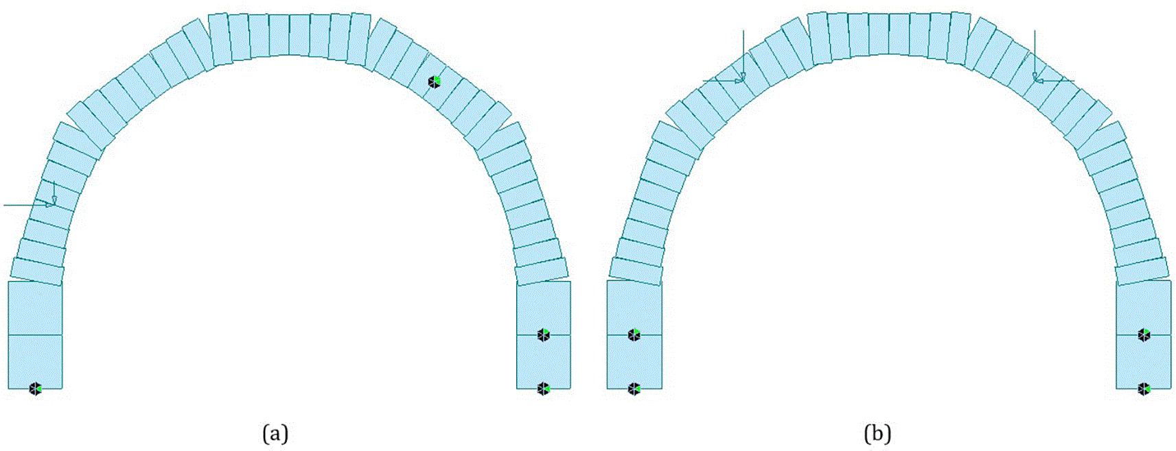
Figure 5. 1D beam model with varying cross-section elements: (a) LC1 and (b) LC2.
Both load combinations were modelled, reproducing the loading and restraining conditions of the mock-ups. As it can be noted in
Figure 5a, for LC1 the legs of the specimen are simply supported and actuators 5 and 7 provide a support for the mock-up, whereas actuator 2 is applying a load which is directed on the centre of the mock-up. Similarly for LC2 (
Figure 5b), the legs are simply supported and actuators 1 and 7 are restraining the mock-up whereas actuators 3 and 5 are applying the load.
For the preliminary model, a linear elastic analysis was performed using the numerical model. The material properties inputted in the model are thus simply the Young’s Modulus (which value of 40 GPa has been computed from Model Code 2010 equation starting from the value of the average compressive strength) and Poisson ratio (assigned of 0.2). The results of interest of the linear elastic analysis are the distributions of the bending moment in the structure for the different loading combinations. Using the obtained bending moment distribution, it is possible to predict the cracking of the mock-up, and thus the placement of the cameras for the DIC analysis. In
Figure 6 the bending moment distributions are reported.
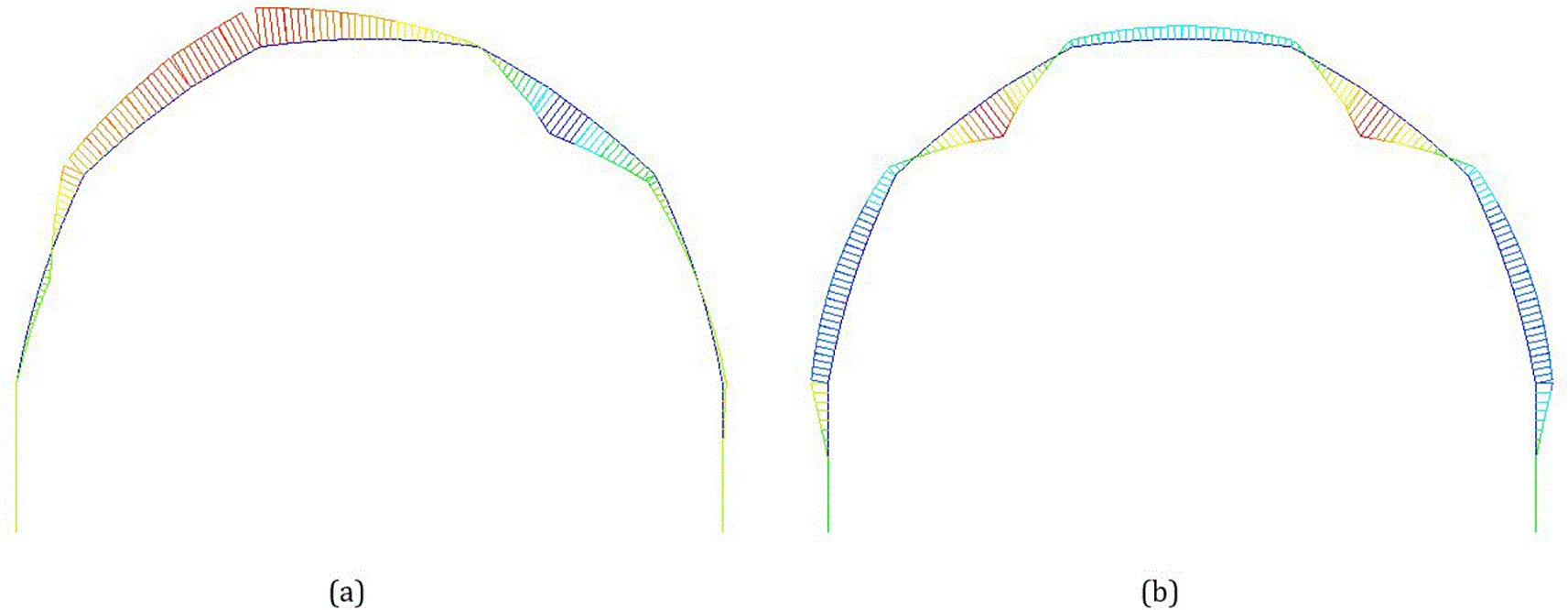
Figure 6. Bending moment distributions for the two different loading combinations: (a) LC1 and (b) LC2.
According to the results of the preliminary numerical model, it is worth noting that for LC1 the bending moment distribution suggests the formation of cracking of the mock-up in correspondence to actuator 5 which works as restraint, as well as in a position on the left of the key, in between actuators 3 and 4. For the LC2, the bending moment distribution remarks a possible cracking formation in correspondence of actuator 3 and 5, which are loading the mock-up. It is evident that for both the loading combinations a crack may form in correspondence of actuator 5. For this reason, it has been decided that the camera adopted for the DIC analyses the region in correspondence to actuator 5.
Collapse of the mock-ups
In this section the collapse of the mock-ups under the two loading combinations will be analysed, starting from the visualisation of the failure mechanism of the specimens and their structural behaviour, up to the study of the cross-sectional behaviour using the DIC analysis.
The failure mechanism of the mock-ups under the different load combinations have been correctly predicted by the bending moment distribution of the preliminary numerical model. In fact, as it can be noted in the collapsed specimen of
Figure 7, the cracking formation position coincides with the predicted bending moment distribution. For LC1 two cracks formed after the collapse of the mock-up, one with the opening on the extrados surface and the other with the opening in the intrados surface (as correctly predicted by the sign of the bending moment distribution). For LC2 three cracks formed after the collapse of the specimen, with the first two “positive cracks” predicted by the bending moment distribution, and a third one generated by a negative bending moment at the key. This last crack has not been predicted by the preliminary model which limits its predictions until the elastic limit of the structure. However, due to the inelastic nature of the specimen, as well as the degree of redundancy, additional cracks may form on the mock-up.
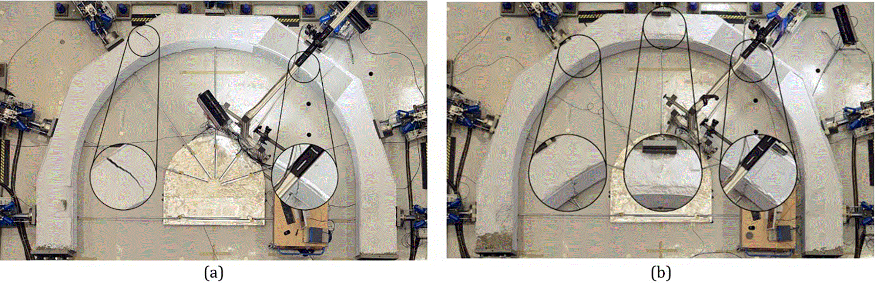
Figure 7. Cracking formation after collapse of the mock-ups: (a) LC1 and (b) LC2.
With the aim of visualising the structural behaviour of the mock-up for the different load combinations, the load-displacement curves in
Figure 8 were obtained.
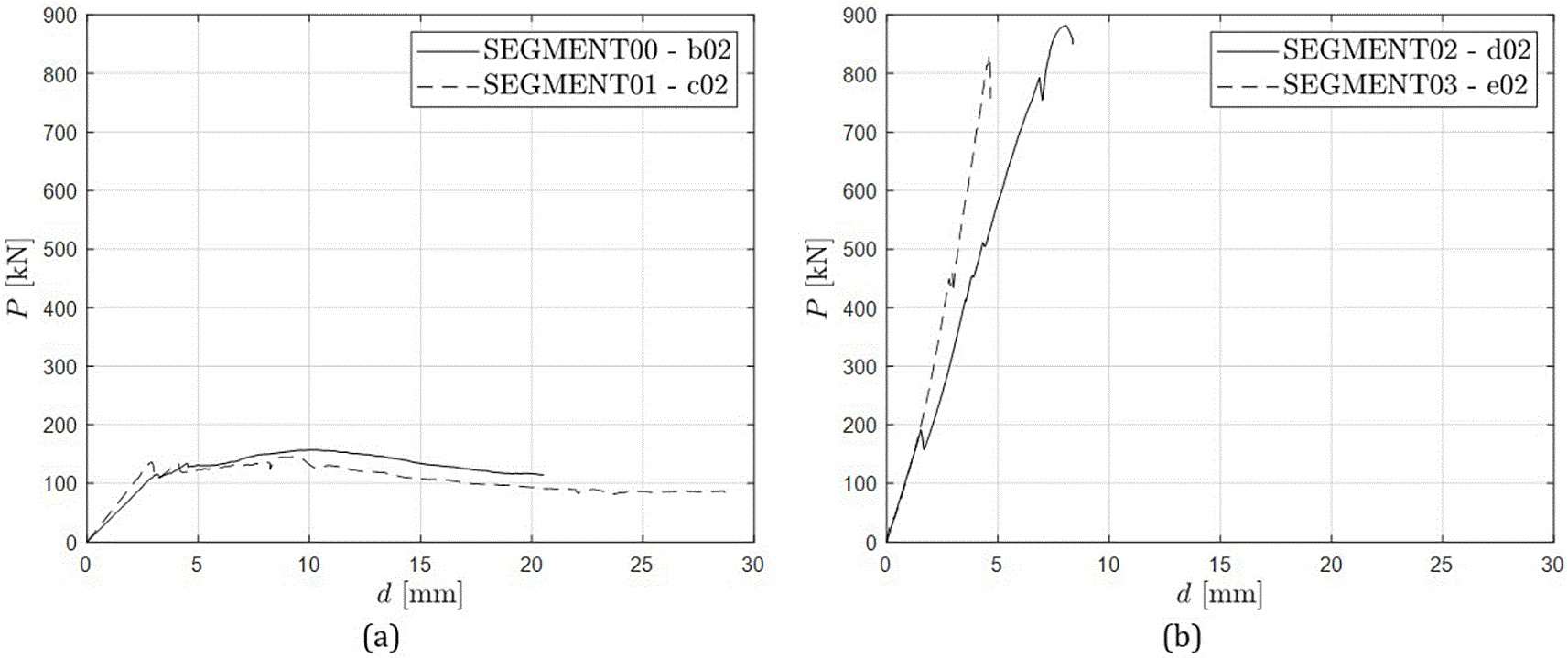
Figure 8. Load versus displacement curves for (a) LC1 and (b) LC2.
For both load combinations, the mock-up was able to increase the value of the load after the formation of the cracks. For LC2, due to the larger compressive stresses in the structure, the hardening behaviour is more pronounced, as the ultimate load achieved by the specimen is much higher compared to the one obtained in LC1. In the latter case, the confinement pressure induced by the load combination is almost zero, as the static scheme does not favour the arch effect as for LC2. For this reason, in LC1 the post-cracking behaviour of the structure is entirely provided by the fibre reinforcement in the cracked cross-sections.
Digital Image Correlation
As previously discussed, the cross-section analysed using DIC is the one in correspondence to actuator 5, in the proximity of which a speckle pattern has been applied (see
Figure 3b). During the tests, the camera acquired images at a frequency of 0.2 Hz, and their analysis was made possible using the “ncorr” plug-in of the commercial software Matlab.27 The software processes the sequence of frames and studies the variation of speckle position with respect to the reference frame (in terms of pixels) in order to develop the displacement and strain fields for each frame for a specific Region Of Interest (ROI) selected by the user. Finally, the calibration frame ensures conversion from pixels to millimetres. For this specific experimental campaign, only the DIC analyses for mock-up 2 and 3 are available.
Through the DIC analysis it is possible to study the displacement field of the region of interest for each frame. From the displacement field it is thus possible to visualise and quantify the crack opening during the test. It is thus meaningful to select specific limit states for the quantification of the crack opening. For example, one may define the limit states with respect to the total displacement computed by the loading actuator. In this case, six limit states have been defined, as percentage of the final displacement: in particular five limit states have been identified corresponding to 20%, 40%, 60%, 80% and 100% of the final displacement (namely LS1, LS2, LS3, LS4 and LS5), and a sixth limit state corresponding to the formation of the crack (identified as LScr). In
Figure 9 the displacement field contour plot are reported, referring to a non-dimensional ROI defined by the
and
coordinates, which assume values varying from 0 to 1.
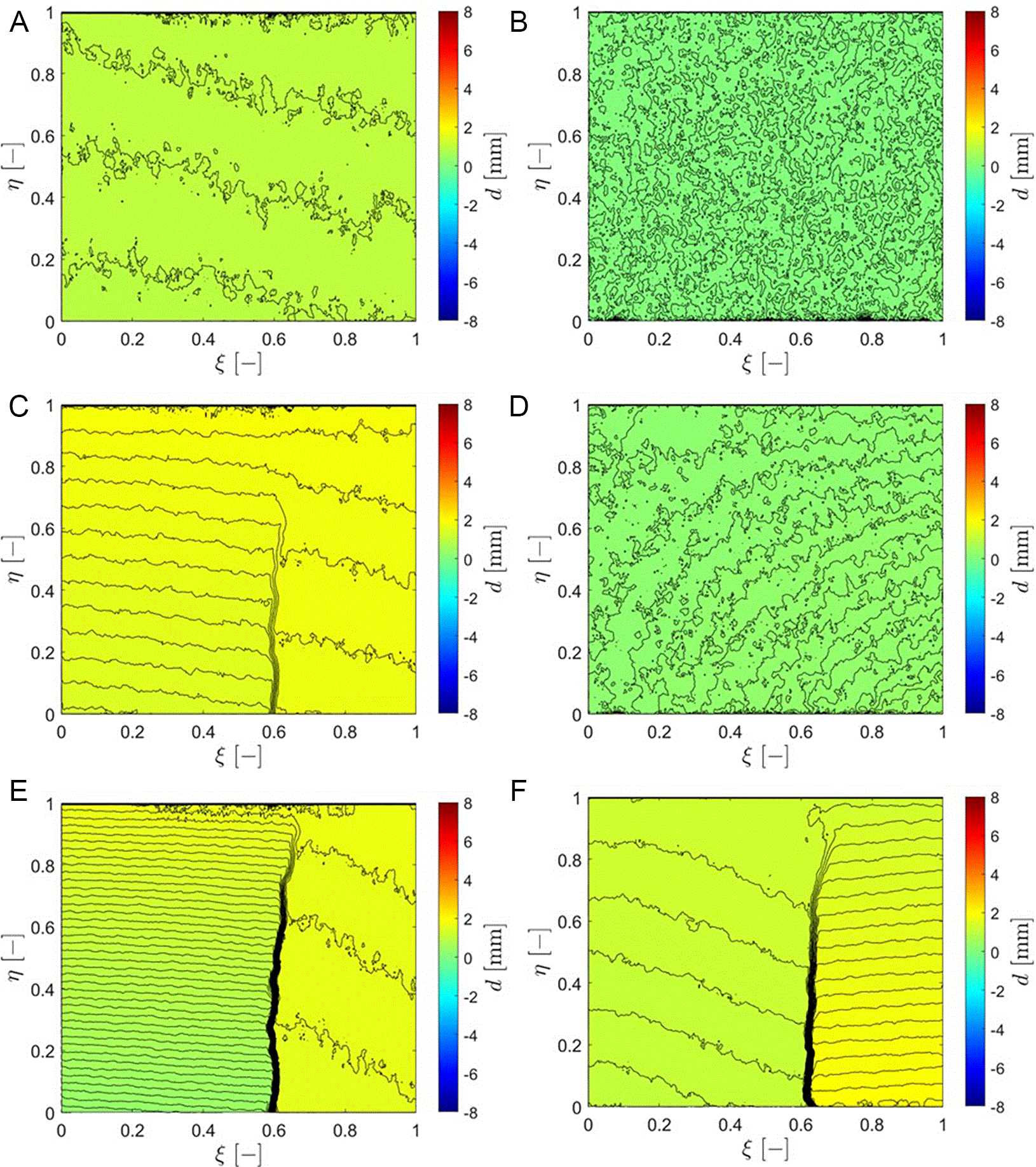
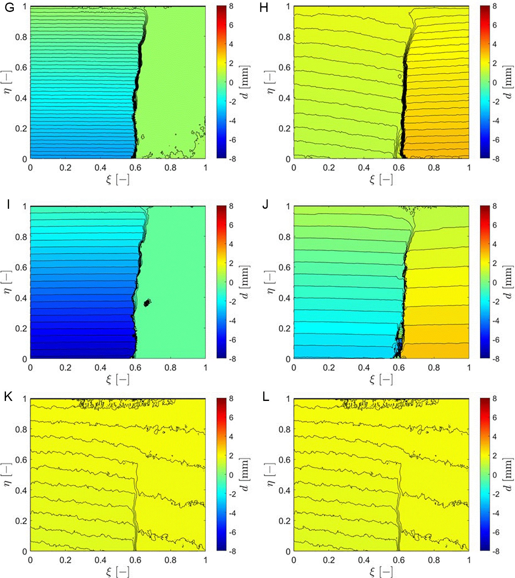
Figure 9. Displacement fields for the different limit states. Figures (A)-(C)-(E)-(G)-(I)-(K) refer to LS1-5 and LScr for Mock-up 2, whereas figures (B)-(D)-(F)-(H)-(J)-(L) for Mock-up 3.
It is worth noting that right after the formation of the crack (LScr), this generates a localised discontinuity in the displacement field. The higher the limit state, the larger the discontinuity in the displacement field. This can also be quantified as crack opening, by simply considering the difference between the displacements of two points on either side of the crack. In particular, it is possible to compute the variation of the Crack Opening Displacement (COD) along the cross-section for each limit state. Defining the cross-section axis as
, which varies between 0 mm (in correspondence of the extrados) and 400 mm (in correspondence of the intrados), the COD profiles in
Figure 10 are obtained.
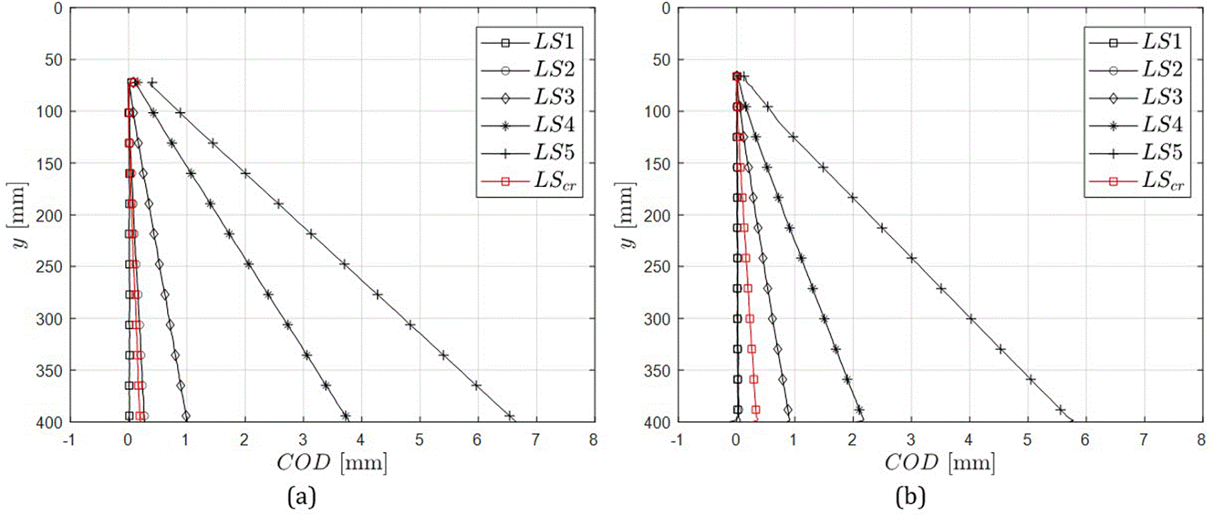
Figure 10. COD profiles along the cross-section height for (a) the mock-up 2 loaded according to LC1, and (b) the mock-up 3 loaded according LC2.
The COD profiles confirm previous observations, as the crack opening evolves with the limit state. Moreover, it is worth noting that the COD varies linearly along the cross-section for each limit state, meaning that the cracked cross-section rotates remaining flat in its plane.
Through the DIC analysis the COD was computed for each image time step, which was related to the load in the curves shown in
Figure 11. Here, the load corresponds to that applied by the loading actuator (actuator 2 for LC1 and actuator 5 for LC2), and the COD corresponding to the one obtained by DIC analysis of the region in proximity of actuator 5 for both load combinations.
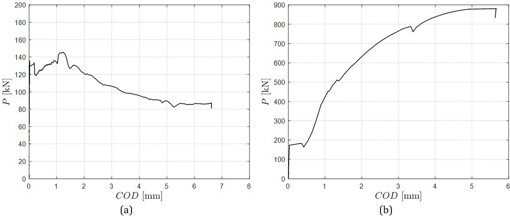
Figure 11. Load versus COD curves for (a) mock-up 2 loaded according to LC1, and (b) mock-up 3 loaded according to LC2.
It is worth noting that for both mock-ups (thus for both load combinations) the fibre reinforcement enhances the structural performance of the specimens. For LC1 the cracking load registered is close to 140 kN, which is lower than the one obtained for LC2 which reaches a value close to 180 kN. After the formation of the crack, the load increases thanks to the residual tensile strength provided by the fibre bridging mechanism. Due to the fibre presence in the mock-ups, the cracked cross-sections have been able to reach high value of COD (close to 7 mm for LC1 and to 6 mm for LC2), keeping the value of the load high. As already examined, the hardening observed in the mock-up 3 loaded by LC2 is much larger than the hardening obtained for the other mock-up. In fact, for LC1 the maximum load achieved is equal to 145 kN, whereas for LC2 the maximum load is equal to 890 kN. This large difference is provided by the confinement effect generated by LC2, induced by the compressive stress distribution in the mock-up, which increases the load required for the failure of the specimen.