1. Introduction
With increasing renewable power generation integrated into the power system, the fluctuations from the supply-side need to be balanced. Demand response (DR) can bring a valuable contribution to the power system by using time of use dependent pricing schemes1. Residential buildings provide promising options for DR, especially the buildings with heat pumps (HP) and thermal storage that can be incentivized to shift loads by a price signal2.
The operation of the HP can be optimized either by an in-house smart energy management system (SEMS) or a remote aggregator meaning that the heating system will be operated not by the homeowner. We will focus on an in-house operation implying that homeowners provide flexibility for their own benefit. In this paper we investigate one of many different incentives that can be used to influence the local control. One straightforward way is to introduce a variable real-time electricity price (RTP). If the prices in the following hours are known, the HP operation can be adapted to the price settings and economically optimize HP operation. Naturally, lower prices will occur when the production of renewable electricity is high, and prices will be higher when there are fewer renewables in the electricity mix3.
Existing studies have evaluated the economic impacts of different pricing schemes on the HP-operated buildings4–6. In most studies, the flexibility is provided by the battery or thermal storage in the building. Flexibility in these studies is defined as the amount of energy (electrical or thermal) that is used at a different time than originally anticipated. In this sense flexibility could be interchangeably used with the term load shifting. As shown in another strand of literature, the load shifting potential of the building’s thermal mass is also significant7,8.
In this study, we combine these two strands of literature and investigate how much the electricity consumption profile can be influenced if we combine variable electricity prices with the SEMS. We consider the flexibility of building mass alone and compare it to the flexibility with implemented thermal storage systems. Two research questions are formulated: How can RTP signals influence cost-minimizing control strategies of residential single family houses (SFH)? Second, what are the implications of variable real-time electricity pricing and in-house SEMS at the national level?
To answer these two questions, our study includes three parts:
First, we developed an hourly technology operation model for individual households by taking a single SFH with a HP installed as an example. Assuming the electricity price, outside temperature, and radiation as input, the model determines the operation of the HP. The model can run in two modes. In the reference mode, the operation of technologies is simulated keeping indoor temperature above a certain level, with the energy consumption and cost calculated accordingly. In the optimization mode, technologies’ operation is optimized to minimize the energy cost.
Second, we developed multiple scenarios for variable electricity prices following the RTP mechanism based on the Balmorel model9,10. The modeled prices reflect different scenarios with increasing marginal costs for power plants that provide flexibility. This way, we investigate how price volatility influences the incentive for load shifting.
Third, by linking to the INVERT/EE-LAB11 building stock model, we aggregate the results of individual households to the building stock level and explore the impact of RTP and in-house SEMS on the load shifting potential and the peak demand of the Austrian SFH building stock.
This paper contributes to existing literature by investigating load shifting potential on an hourly level over the whole year taking also future electricity price scenarios into account. Specifically the impact of increased price volatility is investigated. Additionally we show how load shifting measurements could influence the total peak demand on an aggregated level. The remainder of this paper is structured as follows. Section 2 overviews existing studies on HP-operated residential buildings’ flexibility potential and different variable electricity price mechanisms. Section 3 introduces our model in detail and provides the input data and scenario definitions. Then, in Section 4, we present the results by analyzing the impact of various electricity prices on the load shifting behavior and the fiscal incentive. At last, we conclude in Section 5, discuss the limitations of this approach, and point out the need for further research.
2. Literature review
In literature, HP-operated buildings’ economic advantages with a variable price scheme are often discussed in combination with storage applications. Bechtel et al.12 analyze how different buffer heat storage sizes and the HP power impact the cost savings of a HP-operated building with a variable price signal. They find that HP start-ups can be reduced significantly with higher storage capacity. Operation costs can be reduced by up to 20% with a 1500 l buffer storage in an SFH. However, when considering the additional investment costs for the larger storage, a 200 l buffer storage is preferred. The electricity prices used in this particular study are historical prices for the German-Luxemburg market (EPEX Spot). They do not consider different price schemes in this study. In a case study, Fitzpatrick et al.4 compare three different electricity tariffs for a residential building with a combined HP and gas boiler. The house had a 2000 l buffer storage and a 400 l domestic hot water tank. It turned out that the building provided the highest flexibility with the RTP scheme. The other pricing schemes are a two-level day/night tariff and a critical peak pricing with three different price levels depending on the hour of the day. Patteeuw et al.6 on the other hand, showed that dynamic time of use pricing performs inferior in comparison to the direct load control in regards to CO2 savings and cost savings with a high level of residential HP penetration. They assessed the value of load shifting in high-energy-efficient HP buildings. Two load shifting controls are adapted: 1) a direct load control where the HP load is controlled by a third party and 2) real time pricing. They analyzed how load shifting with residential HPs can reduce CO2 emissions and what incentive is best for home owners to participate in load shifting.
Ostergaard and Andersen5 investigated the impact of electricity taxes on the incentive to increase HP power and thermal energy storage. Additionally, they examine the incentive of the alignment of HP operation with the dynamic electricity system needs in a district heating system. Variable taxes (hourly) incentivizes increasing thermal energy storage by 20%. The HP capacity however, is not affected. They do not consider different electricity pricing schemes.
Other studies denote that load shifting through variable electricity tariffs will lead to a higher electricity demand overall13,14. Miara et al.13 states that HP systems in combination with buffer storage provide promising DR possibilities. However, because of heat losses and the increased HP operating temperatures when charging the buffer storage, the electricity consumption increases by 20% when DR is fully exploited. Kelly et al.14 tries to shift all heating loads from peak periods to off-peak periods in a typical detached dwelling in the UK. A 1000 l hot water storage is sufficient, but the overall electricity demand increases by 60%. Additionally, the tank’s charging demand is 50% higher than the average house would have had in the peak period.
Many studies investigating the impact of variable electricity prices focus primarily on load shifting with thermal or electrical storage. However, as widely discussed in existing studies, the thermal inertia of buildings also provides significant potential for load shifting.
For example, Golmohamadi15 creates a stochastic model predictive controller for HP buildings focusing on thermal inertia and heat storage in the building. They find that ambient temperature and electricity price uncertainty has a more significant impact on the economic analysis than the domestic hot water consumption uncertainties. Sperber et al.7 find that the maximum shiftable load in German SFH is 57 GW el by increasing the indoor temperature by 2°C. Weiß et al.8 focuses on the peak shaving potential in the Austrian building stock through thermal inertia. They concluded that 50% of the heating peak loads could be shifted to off-peak hours for buildings built after 1980 by turning off the heating system until indoor temperature is reduced from 22°C to 19°C in a typical winter week. Masy et al.16 find that 3–14% of the heating load can be shifted by using thermal inertia in a single, well-insulated building. While the heat transfer rate between the interior and the thermal mass is low, the amount of energy stored is still impressive. In this regard, Wolisz17 suggests that by pre-heating a building for two hours, the heating demand for the following four hours can be reduced by 20% although the simulated building is made out of bricks and has no insulation. Floor heating and direct thermal activation are more effective in shifting loads with thermal inertia, however HP peak loads can still be significantly reduced with a radiator heating system and the proper control strategy18.
In this work, we dive deeper into the effect of a variable electricity price for buildings operated with a HP. Among different variable electricity price mechanisms (e.g. critical peak pricing, day/night tariffs, or real-time pricing), we focus on the RTP for two reasons: (1) some real-time pricing schemes for residential consumers are already established in Austria; (2) it is a straightforward way to incentivize residents to shift their demand and has been proven to be more effective than other pricing schemes4.
3. Methodology
Model overview
We developed an hourly technology operation model for individual households to model the response of households’ energy consumption to variable electricity prices. The model calculates the operation of technologies throughout a whole year (8760 hours) in two modes: 1) reference mode, in which the energy demand of the building is met to keep a certain comfort level, and 2) optimization mode, in which a SEMS minimizes the operation cost of the household while keeping the same comfort level. Both modelling modes are shown in Figure 1 which also presents the model's general set up. Further details can be found in 191.
Figure 1 presents the model’s general set up - input and output. Further details can be found in 191.
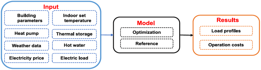
Figure 1. Overall structure of the model.
The relevant parts of the model for this paper are introduced as follows.
The necessary heating demand was calculated with a simplified five resistance one capacity (5R1C shown in Figure 2) approach following the DIN ISO 13790. This norm is outdated and has been replaced by the DIN ISO 52016. But the computational effort to implement the DIN ISO 52016 into the optimization framework is much higher. Both modeling approaches have been compared in 20. And the 5R1C approach has been tested against results from Energy Plus, Invert/EELab and the VDI 600721–23. They show that the heating demand calculated by the 5R1C model is reasonably accurate, whereas cooling demand is strongly overestimated. Bruno et al.24 investigated the thermal dynamics of the 5R1C approach compared to TRYNSIS. Similarly to that study we compared the dynamic behavior of our model to a simulation in IDA ICE2. Our approach with only one capacity underestimates the thermal inertia in general, specifically when there is floor heating, which is quite often the case in SFHs with heat pumps. Therefore, the results obtained by this approach can be seen as a lower benchmark to the actual flexibility potential.
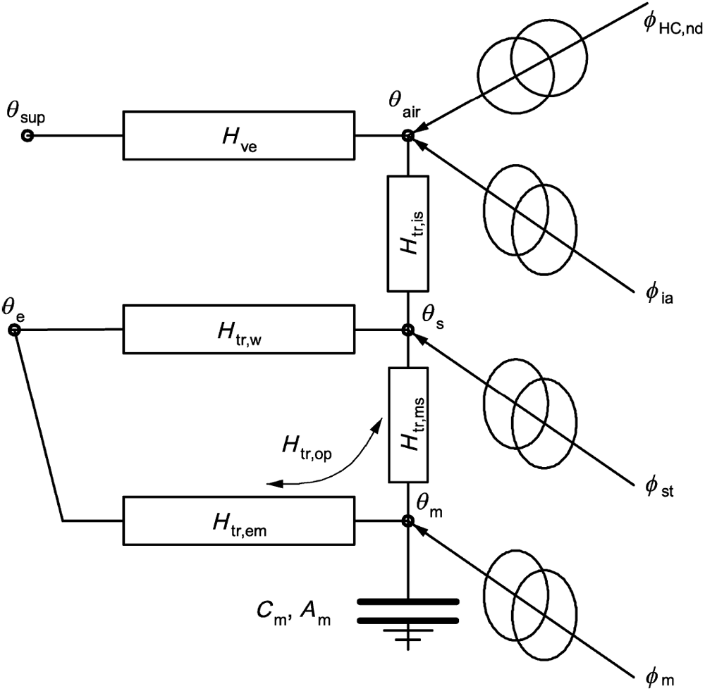
Figure 2. 5R1C circuit representation.
5R1C model
Figure 2 shows the circuit representation of the 5R1C model described in the DIN ISO 13790. The relation between outside temperature (θoutside), indoor temperature (θair) and heating demand (ϕHC) is provided by the following equations. A detailed description of the calculation methodology can be found in the DIN ISO 13790. In the following equations, ϕ represents any kind of heat flow in W and θ is used to describe temperatures in °C. Equation 1 describes the relation between the indoor temperature () and the provided heating energy (). ϕia describes the heat flow from internal gains:
θsup describes the air temperature from the ventilation system. If no ventilation system with heat exchangers is adopted θsup is set to θoutside. In this study ventilation systems are neglected.
ϕint describe the internal heat gains in W/m2. For simplification the internal gains (ϕint) are kept constant with 3.4W/m2, although in reality they can change every hour.
The node temperature θs is calculated through following equation:
The average temperature of the thermal mass () in each timestep is calculated as follows:
and represent the temperature of the thermal mass in the current and in the previous timestep and have to be calculated for each timestep individually:
with the heat flow to the thermal mass node ϕm tot:
The heat flow to the indoor surface node s, ϕst is calculated with
with ϕsol describing the solar gains.
Every parameter described with an H represents a transmission heat transfer coefficient and is given in W/K. All building specific parameters are described in the following equations:
with Hve being the ventilation transfer coefficient.
with his being the heat transfer coefficient between the air node θair and the surface node θs which equals to 3.45W/m2K1. Atot denotes the total surface area of the building in m2.
where Af is the heated floor area in m2 and Λat represents the dimensionless ratio between the surface area of all surfaces that face into the space and the heated floor area. Λat is set to 4.53.
Hop is presenting the heat transfer coefficient through opaque building elements. Hms is calculated with the following equation:
hms denotes the heat transfer coefficient between the nodes m and s and is fixed with 9.1W/m2K1.
Am is the effective mass-related area in m2 and is calculated with following formula:
Aj represents the surface area of the building element j in m2 and kj represents the specific thermal capacity of a building element j in J/m2K. Cm is provided in J/K and denotes the total thermal capacity of the building mass:
HD, Hg, HU and HA represent the transmission heat transfer coefficients for direct heat transmission to the external environment (HD), for the steady-state heat transmission to the ground (Hg), through unconditioned rooms (HU) and to adjacent buildings (HA). The calculation of these four parameters is described in the DIN ISO 13789. In the following equation HX stands for either HD,Hg,HU,HA:
with Ui being the heat transfer coefficient in W/m2K for the respective building element i.
ψ... linear heat transfer coefficient for a thermal bridge
l... length of a thermal bridge
χ... heat transfer coefficient for a punctual thermal bridge
btr,x... adjustment factor if the temperature on the other side of the component is not equal to the temperature of the external environment
The total ventilation heat transfer coefficient (Hve) is calculated as follows:
ρa × ca... volume-related heat storage capacity of the air in J/m3K
qve... the time-averaged air volume flow
bve... the temperature adjustment factor for airflow element k. If the supply air temperature is not equal to the temperature of the external environment, bve ≠ 1.
Heat pump
Space heating and hot water demand are met by an HP where the coefficient of performance (COP) is dependent on the supply and the source temperature (in K):
η represents a constant efficiency factor and is set to 0.35 for air source HP and 0.4 for ground source HP4. For space heating, an average supply temperature (Tsupply) of 35°C was assumed, and for domestic hot water, the supply temperature was 55 °C. If the HP charges a thermal storage, the supply temperature rose by 10 °C. Indoor temperature was set to be within 20°C and 23°C. For the air source HP the source temperature (Tsource) was the outside temperature and assumed to be a constant 10°C for the ground source. The maximal electric capacity of the HP was determined by calculating the necessary thermal power of the building and COP at design conditions. In Austria, design outside temperature is around -12°C26.
Austria’s outside temperature and radiation profile is generated by weighting the profiles for every NUTS35 region in Austria by their respective residential floor area and taking the average. The data is downloaded from PV GIS27 for 2019.
Thermal storages
To determine the influence of thermal storage devices on a building to shift electric loads, we simulated a SFH once without any thermal storage device and once with a buffer storage for heating and a tank for domestic hot water (DHW). The size of the DHW storage was chosen to be 400 l, and the buffer storage for heating had a volume of 750 l. Following assumptions were made regarding the hot water storage to keep the model linear:
The temperature inside the tank is homogenous.
The temperature surrounding (Ttanksurrounding) the tank is constant at 20°C.
Thermodynamic properties of the water (volume, heat capacity (cwater in J/kgK) and pressure) are constant.
The following equations represent the physical limitations of the hot water tanks:
denotes the energy stored in a tank (J) at a particular hour with mwater (kg) being the mass of the water and the current temperature inside the tank. is the minimum temperature inside the tank and was chosen to be 28°C. is the temperature inside the tank at the start of the simulation. The maximum temperature of the buffer heating storage is 45°C and 65°C for the DHW storage. To prevent legionella the DHW tank is regularly heated above 60°C. Both storages have the same insulation with a heat transfer coefficient (Utank) of 0.2 W/m2. The buffer storage and the DHW tank have a surface area (Atank) of 4.6 m2 and 3 m2, respectively. describes the thermal losses of the storage.
In the further course, we simulated multiple representative buildings from the Austrian SFH building stock and aggregated the results to the national level.
Model objective
An optimization was developed in Pyomo28 and solved by Gurobi6 to minimize the household energy cost. The objective function of the model is to minimize the operation costs over one year on an hourly basis:
With Pt being the electricity price and Et the amount of electricity bought from the grid at a certain hour. The electricity consumption is composed of fixed and variable components. Fixed components of the electricity consumption are internal loads from appliances and lighting as well as the electricity demand of the HP for hot water generation in case there is no DHW storage. The electricity consumption profile is a synthetic load profile for a single household7. The hot water demand consumption rate is assumed to be 90 l per day29 with an initial temperature of 10°C and a supply temperature of 55°C. The hourly demand profile is taken from the Hotmaps project30.
The variable electric load consists of the electricity demand from the HP. The SEMS can increase the heating demand in a specific timeframe by pre-heating the building and reduce it in the following hours. Additionally, if the building is equipped with thermal storages, they can be charged and discharged at any time. Thus, the SEMS can shift electricity demand for heating even more effectively.
Similar to 4 shifted energy (Eshifted) in this study was defined as the difference between the electric power consumption profiles with and without DR:
denotes the electric load from the grid in the reference case and the load with a SEMS installed. If is higher than the building is being pre-heated or storages are charged. Likewise the energy is shifted whenever is higher than . Naturally the shifted energy is is lower than the energy used to charge storages and building mass due to thermal losses.
The reference model cannot shift any loads. Heating demand is calculated based on the same 5R1C approach with the assumption that the air temperature inside the building should not drop below 20°C. The HP then provides the needed heating power to keep the temperature at 20°C with the corresponding COP. As there is no non-smart logic on when to fill and discharge a thermal storage based on the variable price, the reference model does not adapt thermal storages.
Austrian building stock
To capture the possible impact of price incentivized load shifting of the Austrian SFH building stock, we coupled our model to the INVERT/EELab building stock model11. In this database, the SFH building stock in Austria is represented by 36 building categories. Each category represents a typical SFH built in a certain time period and its overall thermal insulation properties. The different representative buildings and the installed number of HP in each category are presented in Figure 3. More information about the buildings is provided in Table 1. The appendix ”mon” indicates that the buildings are under protection. Gen2, gen3, and gen4 indicate that these buildings have undergone a certain renovation, with higher numbers representing more recent renovations. We can see that most HPs have been installed in modern buildings. Overall Austria has around 1.55 million SFHs out of which 180 000 have a HP installed8. In 2023, the Austrian federal government implemented strong incentives for exchanging oil and gas boilers with HPs by subsidising installation costs up to 75%.
Thus it is expected that the share of SFHs with a HP will increase significantly within the next years9. Thus, it is expected that the share of SFHs with a HP will increase significantly within the next years. However, in the following analysis we did not change the total amount of heat pump operated buildings nor the characteristics of the building stock itself. Otherwise the resulting shifted electricity would heavily dependent on the chosen building stock scenario and not on the electricity price itself. From Figure 3 we can see that most buildings with heat pumps installed are modern buildings. The chosen 35°C for the supply temperature for all buildings is too low for the old buildings. This simplification however, does not change the results. A higher or lower efficiency of the heat pump reflects itself in the annual heating costs of a building and can therefore also be interpreted as a change in mean electricity price. For the optimization however, only the relative change from one hour to another in price is relevant.
Complete data on the buildings including window areas are provided in 31 in the "Variable\_Price\_Paper.sqlite" file under the table name "OperationScenario\_Component\_Building".
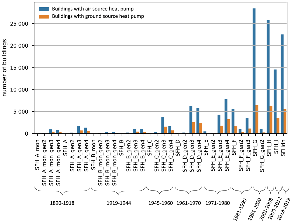
Figure 3. Number of buildings with HPs ins the Austrian SFH building stock11.
Table 1. Building IDs with 5R1C parameters11.
| ID | Name | Generation
of renovation | Age class | Af (m2) | Hve | Hop | Htr,w | Cm (mio. J/K) |
|---|
| 1 | SFH A mon | - | 1890–1918 | 129 | 36 | 229 | 101 | 53 |
| 2 | 1 | 242 | 87 |
| 3 | 2 | 250 | 78 |
| 4 | 3 | 198 | 76 |
| 5 | SFH A | - | 1890–1918 | 129 | 36 | 227 | 101 | 53 |
| 6 | 1 | 241 | 87 |
| 7 | 2 | 250 | 78 |
| 8 | 3 | 164 | 67 |
| 9 | SFH B mon | - | 1919–1944 | 136 | 38 | 290 | 116 | 46 |
| 10 | 1 | 306 | 100 |
| 11 | 2 | 316 | 89 |
| 12 | 3 | 206 | 78 |
| 13 | SFH B | - | 1919–1944 | 136 | 38 | 288 | 117 | 46 |
| 14 | 1 | 305 | 100 |
| 15 | 2 | 316 | 89 |
| 16 | 3 | 189 | 74 |
| 17 | SFH C | - | 1945–1960 | 144 | 41 | 278 | 116 | 31 |
| 18 | 1 | 295 | 99 |
| 19 | 2 | 304 | 89 |
| 20 | 3 | 183 | 70 |
| 21 | SFH D | - | 1961–1970 | 154 | 44 | 193 | 95 | 33 |
| 22 | 1 | 206 | 82 |
| 23 | 2 | 212 | 77 |
| 24 | 3 | 150 | 68 |
| 25 | SFH E | - | 1971–1980 | 163 | 46 | 204 | 101 | 35 |
| 26 | 1 | 214 | 90 |
| 27 | 2 | 226 | 79 |
| 28 | 3 | 159 | 71 |
| 29 | SFH F | - | 1981–1990 | 166 | 46 | 141 | 79 | 35 |
| 30 | 1 | 149 | 71 |
| 31 | 2 | 142 | 69 |
| 32 | SFH G | - | 1991–2000 | 170 | 48 | 120 | 71 | 31 |
| 33 | 1 | 122 | 68 |
| 34 | SFH H | - | 2001–2008 | 170 | 48 | 90 | 59 | 19 |
| 35 | SFH I | - | 2009–2012 | 170 | 48 | 87 | 62 | 19 |
| 36 | SFH dh | - | 2012–2019 | 170 | 48 | 59 | 47 | 19 |
Electricity price scenarios
The electricity price is the driving factor of the energy cost minimization problem. In future decarbonized electricity systems, a higher price variance on electricity spot markets is expected for systems with very high shares of renewable generation3. This is because of more hours with spot prices close to zero due to very high shares of renewable generation with low variable generation costs. In times of low renewable generation and high load on the other side, flexibility options at higher costs like dispatchable generation units, storage discharge, or import set the marginal price, which results in relatively high spot prices. The Austrian electricity system for 2030 was modeled with the bottom-up energy system model Balmorel9,10 to reflect such a decarbonized power system with higher price variance. In Balmorel we modeled the Austrian electricity and district heat system as well as the neighboring countries Czech Republic, Germany, Hungary, Italy, and Slovenia to capture export and import dynamics. Installed generation capacities, national electricity demand, and net transfer capacities were based on the Ten-Year Network Development Plan (TYNDP) 2020 National Trends scenario.10 For Austria, the assumptions were based on the national energy and climate plan WAM scenario11 and were refined to reflect the 100% renewable target (nationwide in annual balance terms) until 2030. That means that Austria meets its goals defined in the renewable expansion act32 and becomes a net exporter of electricity. The installed capacities in Austria for these simulations are depicted in Table 3 in the Annex. All electricity generated by natural gas is exported (on annual balance). The model with input parameters has been tested and validated in 33,34. Within these system boundaries, electricity demand and supply are matched within a market model, considering supply costs following the merit order principle under the assumption of a perfectly competitive market. It is not determined specifically in which type of market the transactions take place economically. The marginal cost of supplying power demand are derived which can be interpreted as the geographically specific market price of power in the model output.
The aim is to reflect various electricity market settings where different price patterns occur. We modeled three price scenarios to analyze sensitivities differing in the assumed CO2 price. The CO2 price influences the high-price hours when gas-fired units in this system define marginal costs. However, this could be any other flexibility option (eg. hydro pump storage) at a high price level in a different market setting. It should be noted that the flexibility provided by the HPs in the building stock were not considered in the Balmorel calculation. An investigation of the impact of HP flexibility on the electricity price was done in 3.
In total four different electricity profiles were investigated in this study to establish a relation between the volatility of the electricity price and the shifted load by the building. The first profile is Austria’s actual day-ahead electricity spot price 2021 from ENTSO-E12. The other three prices were modeled with Balmorel. To every price profile a hypothetical fixed grid fee plus taxes of 20 cents/kWh were also added in order to derive the retail electricity price.
The resulting mean plus standard deviation for all price profiles are provided in Table 2. With an increasing CO2 price, the price profile’s mean value and volatility increase. All prices are depicted in Figure 4. The sharp increase in Price scenario 1 is due to the gas shortage at the end of 2021.
Table 2. Mean and standard deviation of the price scenarios and CO2 price as well as the number of local maxima in the profile.
Price
scenarios | mean
(cent/kWh) | CO2-price
(€/tCO2) | Number of
local maxima |
|---|
| Price 1 | 30.69 ± 7.76 | - | 1225 |
| Price 2 | 26.05 ± 2.27 | 53 | 621 |
| Price 3 | 28.87 ± 3.52 | 106 | 646 |
| Price 4 | 34.11 ± 6.35 | 212 | 618 |
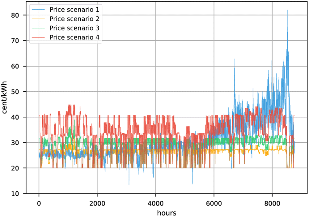
Figure 4. Electricity prices.
In Figure 5 the daily peak-to-peak amplitude difference of all four prices is visualized. The peak-to-peak difference13 in the day ahead price from 2021 increases drastically throughout the year. In the modelled prices for 2030 incisive events, like energy shortages, are not considered, thus the prices were not fluctuating that much throughout the year.
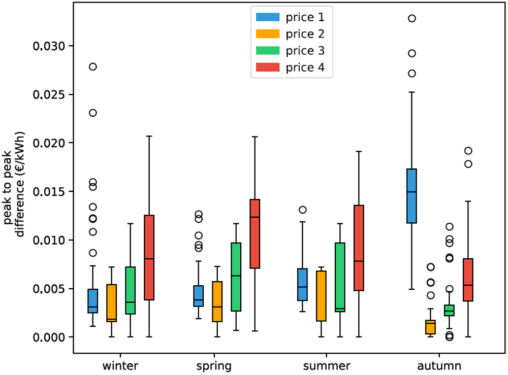
Figure 5. Box plots of seasonal effect in electricity price based on daily peak-to-peak amplitude difference.
Box plots show the median (horizontal line) and the interquartile range (IQR) (box outline). The whiskers extend from the hinge to the highest and lowest values within 1.5 × IQR of the hinge, and the points represent the outliers.
Another significant difference between the 2021 real time price and the simulated prices is the frequency of change. It is visible in Figure 4 that price 1 is changing more frequently than the others. Table 2 shows the number of local maxima in the respective price profiles. The price from 2021 has about twice as many peaks as the prices from 2030 (price 2, 3 and 4). In this work, we focus on volatility in terms of price spread. Structural price volatility in the form of higher frequency can also significantly impact the potential of load shifting. Studies showed that HPs could participate in the intra-day and even the frequency regulation market35,36. But in order to participate in the regulation market they need to be pooled in order to reach the necessary capacity37. In this study we do not consider participation of residential HPs other than the day ahead market. Thus price frequencies are limited to hourly changes. Although the thermal inertia of a building is slow, high frequency of price change generally results in higher cost savings for HPs if they react to the price signal.
Another factor that drives the optimization is the outside air temperature in case of an air source heat pump. However, the change in COP due to the change in source temperature is negligible in comparison to the electricity price when it comes to load shifting incentive.
In the following chapter we will first present the results on single building level before moving to the aggregated results on national level. The single building chosen to investigate the single load profiles is a typical modern SFH in the Austrian building stock, built after 2010. The building has a floor area of 170 m2 and a useful energy demand for space heating of 45 W/m2. The thermal capacity of this building is low and the insulation level high compared to older buildings in the building stock. Then the same building is simulated with a 400l DHW storage and a 750l space heating buffer storage to show the difference in load shifting potential by implementing thermal storages.
4. Results and discussion
The data for all results describe in the following chapters is available at 31.
Results of individual households
In this section, the effects of different RTP schemes on an individual household optimization are analyzed.
In Figure 6 the grid electricity demand for a household in the 12th week is visualized. The three load profiles represent the load if no load shifting is happening (reference), load shifting without any thermal storage (SEMS no storage) and load shifting with a DHW and heating buffer storage (SEMS with storage). On the right-hand y-axis, we see the electricity price profile. We chose the 12th week because during this period price 1 is similar to prices in the years prior to 2021.
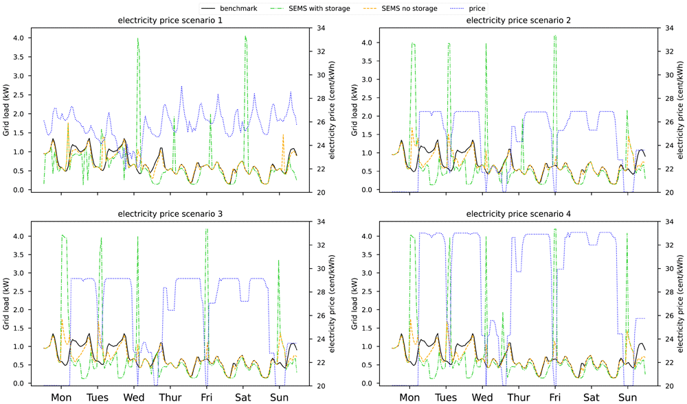
Figure 6. Electricity bought from the grid with and without SEMS in the 12th week of the year.
The electricity price is visualized on the right-hand axis.
Looking at the price scenarios 2, 3, and 4 we see that the higher price difference only increases the incentive to shift loads marginally when thermal storages are available. A change of 6 cent/kWh is enough to charge the thermal storages with the HP. Without thermal storage the peak loads during low energy price times, are limited by the maximum indoor set temperature. With higher price volatility the building is pre-heated to a greater extend if possible.
Figure 7 shows the amount of electricity bought at a specific price. In the reference case electricity is bought independently from the price. But when the household was optimized, electricity was bought at lower prices and demand was reduced at higher prices. In price scenarios 2,3, and 4 the amount of electricity purchased from the grid when the price is at its lowest almost doubles when the household has the thermal storages implemented. Even without thermal storage, the increase in electricity consumption at lower prices and the decrease at higher prices are visible.
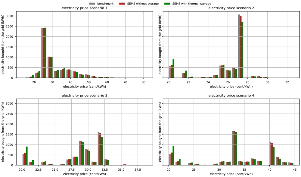
Figure 7. Electricity demand at certain prices in the reference case and with the implementation of SEMS.
”With thermal storage” indicates that the house has a 750 l buffer storage and a 400 l DHW storage.
The maximum average indoor set temperature was varied between 23, 25, and 27°C during winter to investigate the sensitivity of the allowed indoor set temperature bandwidth for pre-heating. Figure 8 shows that higher electricity price volatility increases the incentive to shift energy by pre-heating the building. Comparing the price scenarios 1 to 2,3 and 4, we see that price 1 creates a greater incentive to shift load than price 2 and 3 without the thermal storage. This is due to the nature of the price profiles. Price 1 is changing much more frequently than the other 3 prices. But with the implementation of thermal storages shifted demand is much higher in the price scenarios 3 and 4 and even in price 2 the shifted energy is almost as high as in price 1. The thermal storages compensate for the lower frequency of price changes by storing much more energy in a short period of time. The correlation between the allowed indoor temperature bandwidth and the energy shifted by the optimization is not linear because of the increase in thermal losses with higher indoor temperatures.
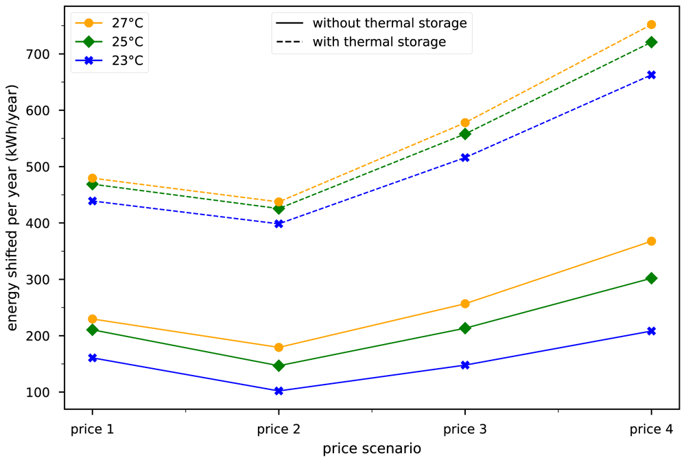
Figure 8. Energy shifted over one year in the building with no thermal storage and the building with DHW storage and buffer storage.
The temperatures represent the maximum allowed indoor temperatures during winter.
If the building has installed thermal storages, the shifted energy rises to around 450 kWh/year in the first price scenario. This result is in line with 4 where a building with 310 m2 floor area, 2000 l buffer storage, and 400 l DHW storage shifts a maximum of 1370 kWh of electric energy. The allowed indoor temperature is still impacting the total amount of shifted load even though the load shifting is done predominantly by the storages. The amount of energy that is shifted with the implementation of thermal storages is by a multitude higher in this case. The absolute amount of shifted energy through thermal storages is almost independent of the building type. Buildings with higher thermal mass and higher energy need, can shift more electricity through the thermal mass. However thermal storages are always prioritized for load shifting because the losses are smaller. Thus any price change which would incentivise a house to pre-heat will give an even higher incentive to shift load via the thermal storage. Although thermal storages efficiently shift energy with minimal losses, using a building's existing thermal mass provides a low-cost way in terms of investment costs if storages are not already installed.
In Figure 9, the annual operation cost savings for each building type are visualized without any thermal storage. With a higher volatility in price change, the economic optimization of HP becomes more lucrative. The optimization is less lucrative for modern buildings. These buildings are characterized by lower thermal mass and a higher degree of insulation. Thus, they have a much lower heat- and electricity demand. The same reason accounts for the difference between air source and ground source HP since the ground source HP is more efficient. Because of the high volatility in the 2021 price profile at the end of the year, the implementation of a SEMS is more lucrative in the buildings compared to the second price profile. A sensitivity analysis showed, that with prices prior to 2021, economic gains through the SEMS were always lower than in the second price scenario. The annual operation cost reductions are generally between EUR 2 and EUR 23 depending on the price profile and the energy demand of the house. If these buildings adapt a 750l heating buffer and a 400l DHW storage, the cost reductions would rise between EUR 5 and EUR 95 without taking any investment costs into account. Therefore, implementing a SEMS into buildings that would use only the thermal mass storage for demand shifting must be very cheap (between 10€ and 100€, depending on the building type) to yield return of investments after, for example five years. Without additional monetary incentives, homeowners are unlikely to tap into the potential of load shifting through the thermal mass alone. This finding is in accordance with other studies that suggest that the additional investments by individual buildings will not be compensated by participating in DR38.
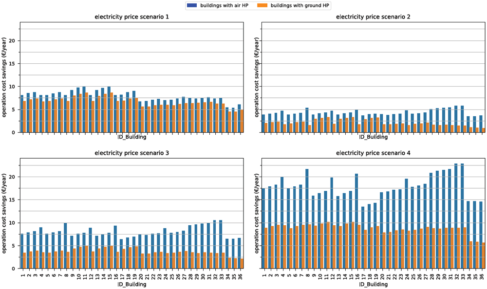
Figure 9. Operation cost savings per building type and HP type in all four electricity price scenarios.
Upscaling to the building stock
In this section, the potential load shift for the whole SFH building stock in Austria is presented in dependence on the four electricity price signals. The used methodology however can be applied to any other European country.
The total amount of electricity shifted over one year in each price scenario is visualized in Figure 10 on the left side. In this case only the thermal mass of the buildings is used for load shifting. The potential of the building stock to shift load via HPs is around 20 GWh when considering the price from 2021. This corresponds to approximately 1.5% of the electricity consumed by these households within the same time period. The increasing volatility in price scenarios 2, 3 and 4 leads to a significant increase in electricity being shifted showing that variable price profiles can give an increasing incentive to shift loads. On the right hand side of Figure 10 the maximum daily peak-to-peak difference of the aggregated load profiles of SFH with HP in the Austrian building stock is visualized. The reference case represents the peak-to-peak demand for the case of no DR. In literature, it is often mentioned that load shifting will result in an even higher peak demand14 14. In the resulting aggregated load profiles, this effect is only marginally visible except in autumn. The electricity price in 2021 was becoming so volatile and high that daily peak-to-peak loads were significantly higher than the reference and all the other scenarios. The peak-to-peak difference of all HP heated SFH buildings in Austria reached a maximum of 350 MW. The peak demand in the Austrian grid was in the magnitude of 80 GW. Therefore potential of the shifting electricity through the thermal mass of SFH was small but not neglect-able.
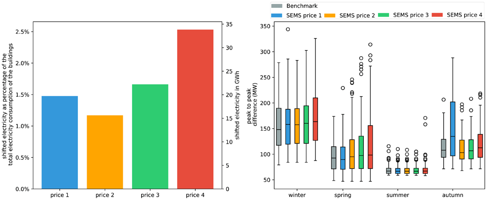
Figure 10.
Left: Amount of electricity shifted throughout the year based on the different price scenarios. Right: Box plots of seasonal effect in grid demand, based on daily peak-to-peak amplitude difference. Box plots show the median (horizontal line) and the interquartile range (IQR) (box outline). The whiskers extend from the hinge to the highest and lowest values within 1.5 × IQR of the hinge, and the points represent the outliers.
As shown before, buildings with implemented storage capacities can shift a lot more electricity. To see how strongly storage capacities can influence the peak-to-peak difference on a daily basis and the overall shifted demand we generated a scenario where every single building with a HP has a 750l heating buffer storage and a 400l DHW storage. The real market penetration of hot water storages in HP operated buildings in Austria is unknown. The following results serve as a reference. In Figure 11 we can see that the peak-to-peak difference is more than two-folding compared to the reference, reaching 700 MW. Also peak demand is reached throughout the year independent of the price scenario. However the occurrence of high peak-to-peak demands increases with increasing price volatility. The total amount of electricity shifted rises to 74 GWh in price scenario 1 which is almost four times higher than without thermal storage capacity.
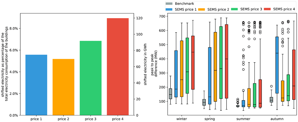
Figure 11.
Left: Amount of electricity shifted throughout the year based on the different price scenarios with buildings having thermal storages. Right: Box plots of seasonal effect in grid demand, based on daily peak-to-peak amplitude difference. Box plots show the median (horizontal line) and the interquartile range (IQR) (box outline). The whiskers extend from the hinge to the highest and lowest values within 1.5 × IQR of the hinge, and the points represent the outliers.
The results show that HPs can effectively shift electricity through the thermal mass. Peak loads increase only marginally for buildings without any storage capacity. Thermal losses that occur when pre-heating a building significantly limit the maximum peak power from an economic perspective when optimizing such buildings’ heating demand. However, with available storages the peak-to-peak demand can more than double. This is especially relevant when HP penetration in a certain region is very high, and HPs are operated with the same strategy. This problem can be avoided by providing different price incentives for users. It is therefore crucial that the price signal reflects electricity scarcity in such a system. Overall the results show that there is significant potential for DR in the residential building stock. This potential can increase even further in the future depending on decarbonisation ambitions and energy scarcity. Furthermore, the potential for the thermal mass is bigger if temporarily cooling down buildings to a certain temperature (e.g. 18°C) is considered as well.
5. Conclusion
The findings in this paper indicate that through the use of RTP in HP operated SFH, large amounts of the electricity can be shifted by the use of thermal mass. An increase in the volatility of such RTP naturally increases the incentive to shift demand. In the year 2021, SFHs in Austria with HPs would shift 19.7 GWh of electricity to lower operating costs if an SEMS was installed without considering any kind of thermal or electrical storages. If thermal storages are considered this amount could be more than doubled. Increasing the volatility of price changes increases the amount of shifted electricity. However, the fiscal incentive to shift demand is unlikely to trigger investments for additional equipment to participate in DR. The installation costs of such an SEMS would strongly impact the decision to implement it. For a single building yearly savings are between EUR 2 and EUR 23 (without thermal storage) and EUR 5 and EUR 95 (with thermal storage) depending on the RTP and the building parameters. Further, we showed that the economic optimization of current buildings in the building stock is slightly more lucrative for buildings with higher energy demand. Comparing the peak-to-peak difference of the resulting profiles in the Austrian SFH building stock with HPs, higher peak loads can be expected when optimizing the HP based on a price profile. However, the effect is limited for buildings without storage devices. Further, the resulting peak loads of individual buildings will have to be compared to the overall electricity demand in the region.
One limitation of this paper is the neglect of changing prices due to load shifting by the buildings. A large penetration of HP-operated buildings that shift loads could lead to a self-cannibalism effect. Further, the possibility of extending the thermal comfort within the buildings down to 18°C for a short period of time would generate additional load shifting potential. The real amount of heating buffer and DHW storages has not been considered for the whole building stock due to the lack of data. Therefore, our results can only serve as a reference to evaluate the impact of SEMS on load shifting. Another aspect that will be considered in further studies are multi family buildings and photovoltaic installations combined with HP. A photovoltaic system would decrease the electricity consumption from the grid and, at the same time, increase the profitability of a SEMS because the SEMS will increase the self-consumption rate of the photovoltaic system.
6. Ethics and consent
Ethical approval and consent were not required.