Implementation of the magnetoelastic extension
To simulate the magnetoelastic dynamics, both the magnetic and elastic equations of motion, i.e. Equation (1) and Equation (4), respectively, must be solved simultaneously. For the implementation, the two first order differential equations in Equation (5) were chosen instead of the the single second order differential equation in Equation (4) for stability reasons. Hence, the system of equations that must be solved becomes
which can be written in a compact manner as
with w = [mx, my, mz, ux, uy, uz, vx, vy, vz] and R = [Tx, Ty, Tz , vx, vy, vz, ax, ay, az]. Note that the magnetic torque T and the effective body force feff include the magnetoelastic field and the magnetoelastic body force, respectively, to account for the mutual interactions between the elastic and magnetic domains. Hence, instead of solving a single differential equation, i.e. Equation (1), the magnetoelastic module must solve a set of differential equations, including elastic and magnetoelastic interaction terms, as a function of time.
Time integration. The time integration of Equation (13) has been numerically implemented via the fourth order Runge-Kutta (RK4) method given by
where the subscript i corresponds to the number of the time step with length ∆t. The k-parameters are given by
To use this new solver instead of the regular MuMax3 solvers that integrate only Equation (1), the user must specify SetSolver(9) in the .mx3 script. The regular MuMax3 solvers run by default with adaptive time stepping. By contrast, the novel solver only runs with a predefined fixed time step ∆t, which also needs to be defined by the user in the .mx3 script. Typical time steps that give accurate results and lead to reasonable simulation times are of the order of ∆t ≈ 0.1 ps. The user can also always verify whether the chosen time step is accurate enough by running an additional simulation with a much smaller time step. If both simulations lead to identical results, the chosen time steps are sufficiently small. If the two results differ, the time step should be shortened further.
Calculation of R. For every time step i, the right hand side of Equation (13), R(t, w), needs to be calculated several times. The vector R comprises the magnetic torque T, the velocity v, and the acceleration a. The numerical calculation of T is already implemented and optimized in the regular MuMax3 framework. Hence, the calculation of T is kept untouched in the magnetoelastic extension. The velocity vector v is obtained by the Runge-Kutta integration of Equation (12). Finally, the acceleration a is determined by calculating a = (feff − ηv) /ρ using the previously found velocity v in combination with Equation (7) and Equation (8), whose sum is the effective body force.
In the following, the numerical implementation of the elastic body force will be explained in more detail since it is nontrivial in presence of free elastic boundary conditions. The elastic body force depends on second order spatial derivatives of the displacement, as indicated by Equation (6). These spatial derivatives are approximated using the finite difference method. In the bulk of the system, the derivatives are calculated based on the sum of a second order forward and second order backward finite difference using averaged stiffness constants. This is done to properly account for parameters that may vary between different positions (regions). To illustrate this approach, the implemented equations to calculate the second order derivative of u(i, j) at position (i, j) with respect to x and the mixed derivative with respect to x and y are
The second derivative in the y-direction as well as the mixed derivative with respect to y and x directions are defined in an straightforward analogous way. For uniform stiffness constants, i.e. c(i, j) ≡ c, these equations reduce to the regular central finite difference scheme, i.e.
and
Boundary conditions. At the edges of a structure, elastic boundary conditions need to be considered, which alter the differential equations and thus their numerical implementation. Three different elastic boundary conditions are implemented in the magnetoelastic module:
1. Periodic boundary conditions, which connect the left edge to the right edge and the bottom to the top of the structure. These boundary conditions do not represent physical boundaries, and therefore Equation (19) and Equation (20) can be used at the edges as well.
2. Fixed boundary conditions, which also do not require modifications of the bulk finite difference scheme. They can be implemented by defining a region at the boundary with a fixed displacement value (e.g. of 0).
3. Free boundary conditions, which correspond to zero traction force at the surfaces.
The third type of free boundary conditions requires the reformulation of the finite difference scheme at the boundaries to satisfy Equation (9). For simplicity, the simulated structure is assumed to be uniform in the z- direction with boundaries only in the x- and y-directions. Moreover, we consider zero traction force. Then, the Neumann boundary conditions at the free surface are
The free boundary condition in the x-direction, i.e. nx = 1, ny = nz = 0, then becomes σxx = σyx = σzx = 0 and similarly for the y-direction, σyy = σxy = σzy = 0.
These expressions must be inserted into the elastic body force at the edges. The implementation of the equations at the mesh edge perpendicular to the x-direction is described below as an example. The same procedure can be used to derive expressions for the corresponding equations at the other interfaces.
The mesh near a boundary in the x-direction is visualized in Figure 2. The interface itself is located at positions (−1/2, j), which are the exact locations where the boundary conditions in Equation (23) are valid. Note that this boundary also describes the limits of the magnetization, i.e. the magnetic material ends at (−1/2, j). By contrast, the coordinates of the points next to the boundary edge can be written as (0, j).
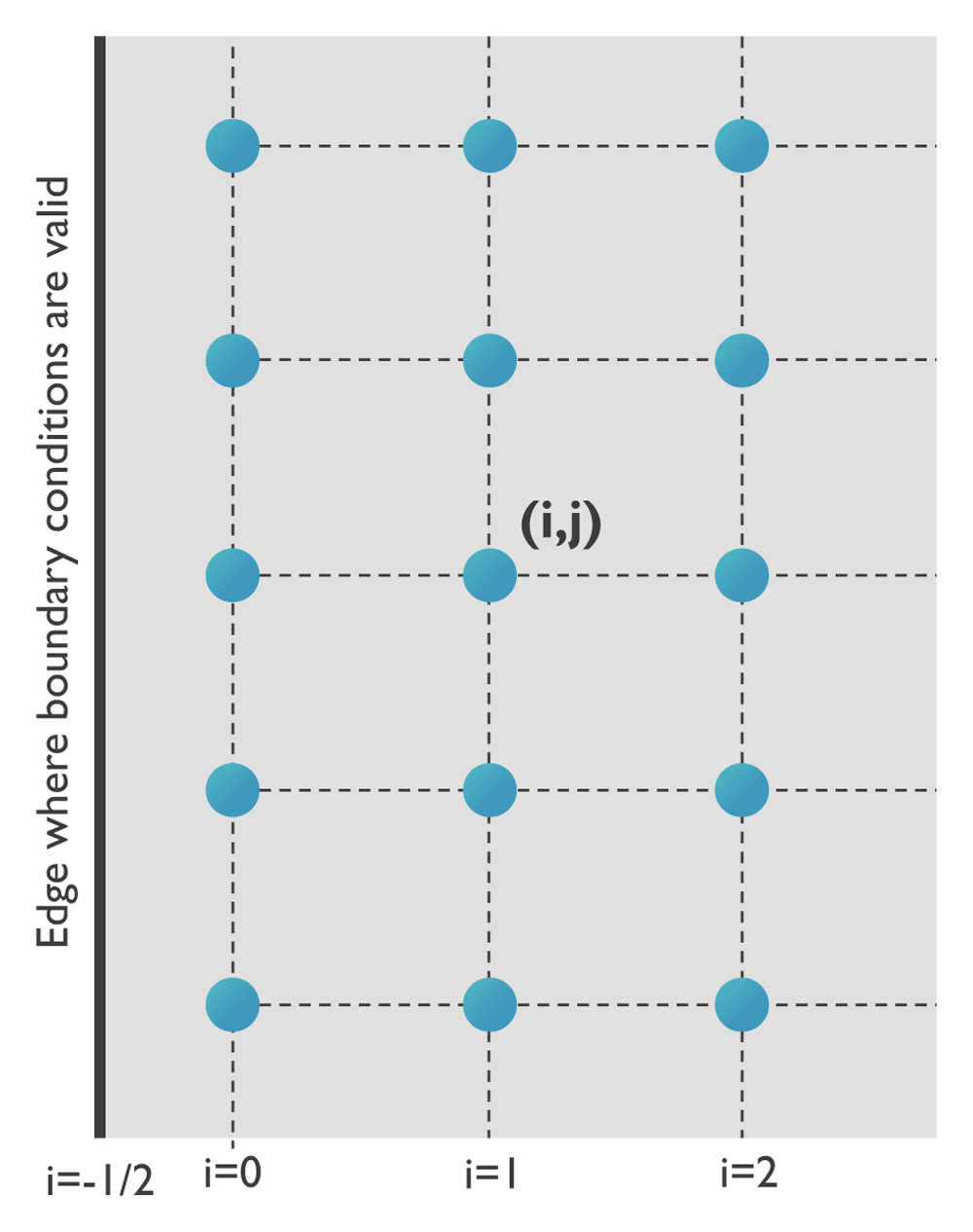
Figure 2. Definition of the grid at a boundary.
For free boundary conditions, the differential equations need to be modified. In the following, the three components of the elastic body force are rewritten in their finite difference approximations taking into account σxx(i − 1/2, j) = σyx(i − 1/2, j) = σzx(i − 1/2, j) = 0.
The x-component of the elastic body force is
At location i = 0, the first term of Equation (24) is given by
with
whereas the second term becomes
Note that the boundary condition formally states that σxy(−1/2, j) = 0, whereas this is approximated by σxy(0, j) = 0 in the numerical implementation. A possible solution to circumvent this approximation is to use a staggered grid where one of the grids contains the displacement values and the other one the stress values. Another solution could be to implement an additional raster of mesh points on the outside of the “original” mesh that can be used to set the proper boundary conditions. In this extension, we have chosen to use the approximation σxy(0, j) ≈ σxy(−1/2, j) = 0 because the mesh is already defined and fixed for the magnetization. However, using another or an additional mesh would strongly complicate the problem since the magnetoelastic extension is built based on the MuMax3 framework, which is designed to work with one mesh only.
The y-component of the elastic body force is given by
Considering again that the surface of the magnetic material is located at i = −1/2 and taking into account the boundary conditions given in Equation (23), the first term can be rewritten as
and the second term as
Finally, the z-component of the elastic body force is given by
In this case, the first term can be rewritten as
and the second term as
Within MuMax3, all these mathematical operations are parallelized and performed on a GPU to reduce the computational time.
Operation of the magnetoelastic extension
The instructions to install the software are provided on the MuMax3 github page https://github.com/mumax/ The software requires the installation of Go and the CUDA Toolkit as well as the availability of an NVIDIA GPU.
In MuMax3, several different data types exist, such as parameters, fields, excitations, etc., which can be defined, modified, or extracted via various methods52,68. This section presents an overview of additional material parameters, vector fields, excitations, energies, boundary conditions, and initial states that are defined in the magnetoelastic extension. Their usage is analogous to the usage of the equivalent elements defined in MuMax352,68 and will therefore be only briefly discussed. Note that all regular MuMax3 methods can also be applied to the new elements defined in the MuMax3 extension.
New material parameters. The usage and the assignment of the newly defined material parameters are the same as for traditional MuMax3 material parameters. Details can be found in the MuMax3 documentation68. Parameters can depend on time and—through the definition of regions—on position. The following list provides an overview of novel material parameters and their units, which are defined in the magnetoelastic extension of MuMax3:
C11: stiffness constant c11 = c22 = c33 of the stiffness tensor with unit [Nm−2];
C12: stiffness constant c12 = c13 = c23 of the stiffness tensor with unit [Nm−2];
C44: stiffness constant c44 = c55 = c66 of the stiffness tensor with unit [Nm−2];
eta: Phenomenological elastic damping constant with unit [kgs−1m−3];
rho: Mass density with unit [kgm−3];
B1: first magnetoelastic coupling constant with unit [Jm−3];
B2: second magnetoelastic coupling constant with unit [Jm−3].
New vector fields. There are two vector field types in MuMax3. The first one is called a variable and can be treated in the same way as the magnetization. The second type is called a quantity and represents a field that can be derived from the fundamental variables. The usage of the new vector fields is the same as for the traditional MuMax368. The novel variables and their units defined within the magnetoelastic extension of MuMax3 are:
The novel quantities and their units defined within the magnetoelastic extension of MuMax3 are:
normStrain: vector that contains the normal strain components [εxx, εyy, εzz], calculated according to , with unit [Nm−2]. Note that the strain corresponds to the real strain and not the engineering strain;
shearStrain: vector that contains the shear strain components [εxy, εyz, εxz], calculated according to , with unit [Nm−2]. Again, note that the strain corresponds to the real strain and not the engineering strain;
normStress: vector that contains the normal stress components [σxx, σyy, σzz], calculated according to Hooke’s law, , with unit [Nm−2];
shearStress: vector that contains the shear stress components [σxy, σyz, σxz], calculated according to Hooke’s law, with unit [Nm−2];
poynting: elastic Poynting vector, calculated via Pel = , with unit [Wm−2];
B_mel: magnetoelastic field µ0Hmel with unit [T] implemented according to Equation (3);
F_mel: magnetoelastic body force with unit [Nm−3] implemented according to Equation (3).
The magnetoelastic MuMax3 extension can simulate magnetoelastodynamics for materials with cubic or higher symmetries. Hence, the module only contains the c11, c12, and c44 stiffness constants. For the strain, the magnetoelastic field, and the magnetoelastic body force, standard central finite difference schemes are used to calculate the derivatives in the respective equations.
Excitations. Excitations, such as applied fields and current densities, can depend on time and space following the form f(t) × g(x, y, z). Here, g can be a continuously varying spatial profile. This is different from the material parameters, which need to be uniform within each region. The following gives an overview of novel excitations and their units within the magnetoelastic MuMax3 extension. Their usage is analogous to the regular MuMax3 usage for excitations68:
force_density: external body force fext that is added to the effective body force feff = fel + fmel + fext, with unit [Nm−3];
exx: εxx strain component;
eyy: εyy strain component;
ezz: εzz strain component;
exz: εxz strain component;
exy: εxy strain component;
eyz: εyz strain component.
Energies. Energies can be extracted at different moments in time to study the system. Every energy contribution can be extracted as either a field or a scalar value. The field corresponds to the energy density and the scalar object corresponds to the total energy of that contribution inside the system. The following list gives an overview of novel energies and their units defined in the magnetoelastic MuMax3 extension:
Initial states. Three new initial states have been implemented for both magnetization and displacement. Their usage is equivalent to the standard MuMax3 usage for the definition of the initial state68.
A Gaussian pulse with spherical distribution of the out-of-plane vector component: GaussianSpherical_outplane(A, pos_x, pos_y, sig_x, sig_y float64), implemented as
A Gaussian pulse with spherical (symmetric) distributions of the in-plane vector components: GaussianSpherical(A, pos_x, pos_y, sig_x, sig_y, angle float64), implemented as
Uniformly oriented in-plane vector components along a specific direction with a Gaussian distribution along the transverse direction GaussianUniform(A, pos, sig, angle1, angle2 float64), implemented as
Boundary conditions. It is possible to apply several types of elastic boundary conditions in the new magnetoelastic MuMax3 module. All elastic boundary conditions correspond to interfaces in the x- and y-directions of the film since uniform displacement is assumed along the z-direction.
Free boundary conditions, corresponding to zero forces at the edges of the film. These are the default boundaries in the x- and y-directions of the film.
Periodic boundary conditions, which can be enabled in the same way as in the traditional MuMax3 framework via the SetPBC() command68.
Absorbing boundaries, which can be implemented by defining regions with gradually increasing elastic damping η, similarly to the gradually increasing damping used to absorb spin waves in a purely magnetic system70. This is, for example, useful to prevent wave reflection at surfaces or interfaces.
Fixed boundary conditions for the displacement are also possible. Such boundary conditions can be obtained by defining regions at the edges of the mesh with fixed displacement values. The parameter frozenDispLoc defines a region with fixed displacement, and the parameter FrozenDispVal defines the fixed displacement value. This works in the same way as the regular frozenspins function in MuMax3, which fixes the spins in a specific region. However, spin (magnetic moment) has always the same norm, whereas the norm can vary for the displacement. Therefore, the additional function FrozenDispVal has been defined. Note that this value can be time dependent and thus can also act as an excitation source.
For example, the code
defregion(2,rect(400e-9,
     1000e-9).transl(-1500e-9,-1000e-9,0))
frozenDispLoc.SetRegion(2,1)
frozenDispVal.SetRegion(2,0,0,0))
sets region 3 to zero displacement. It is also possible to define a time-varying displacement in this region:
defregion(2,rect(400e-9,
     1000e-9).transl(-1500e-9,-1000e-9,0))
frozenDispLoc.SetRegion(2,1)
frozenDispVal.SetRegion(2,
     vector(0.1e-13*sin(2*3.1415*1e9*t),0,0))
This code therefore acts as as a source of (magnetoelastic) waves.