In this section, we present the datasets used for the experiments, the parameter settings, the setup for the experiments, and finally, the results obtained. The source code of the experiments is available in the GitHub repository9.
5.1 Experiments for tabular data classification
In this subsection, we describe the two experiments that we have developed to analyze the utility of data reduction for classification tasks with tabular datasets. In the first place, we detail the methodology to apply the different data reduction methods to a dataset and measure its efficiency, representativeness and performance. Then, we give some details about the two datasets we used. Finally, we show the results obtained for both experiments and discuss the main conclusions.
5.1.1 Datasets for classification
The two datasets that we have used in our experiments are:
Collision dataset This tabular dataset, generated for article 57, was provided by their authors. It can be downloaded from the repository9, which also contains the code for the experiments and our results. The classification task consists of predicting whether a platoon of vehicles will collide based on features such as the number of vehicles and their speed. The dataset consists of 107,210 examples with 25 numerical features and 2 classes:
collision = 1, with 69,348 examples.
collision = 0, with 37,862 examples.
We decided to use this dataset to test the usefulness of data reduction methods to reduce resource consumption in a task related to safe mobility. Before the experiments, we discarded the two features “N” and “m” since they are constant and do not help us in the classification task.
Dry Bean dataset This dataset (see 58 and 59) was created by taking pictures of 7 different types of dry beans and calculating some geometric features from the images, such as the area, the perimeter and the eccentricity. The classification task consists of predicting the type of dry bean based on these geometric features. The dataset contains 13,611 examples with 16 features and 7 classes:
Barbunya, with 1,322 examples.
Bombay, with 522 examples.
Cali, with 1,630 examples.
Dermason, with 3,546 examples.
Horoz, with 1,928 examples.
Seker, with 2,027 examples.
Sira, with 2,636 examples.
The classes were encoded from 0 to 6 for the experiments following the listed ordering. We decided to use this dataset to test the usefulness of data reduction methods for classification tasks with several unbalanced classes.
5.1.2 Methodology
The methodology of the experiments for both datasets consists of the following three steps:
1. Dataset preprocessing:
It is a common practice to scale or standardize a dataset before building the DL model because this increases the likelihood that the training process will be fast and will not be conditioned by some features simply due to their greater magnitude60,61. In our case, we decided to apply the scikit-learn function MinMaxScaler62.
Each feature pj has a maximum value pj,max = maxxi∈X pj(xi) and a minimum value pj,min = minxi∈X pj(xi). We say that the range of pj is the interval [pj,min, pj,max] because all its possible feature values lie in it. Rescaling with MinMaxScaler is just changing each example xi ∈ X by:
After scaling, the range of all the features is [0, 1]. That means that all of them have similar values and can be compared between them.
2. Fixing the architecture and hyperparameters:
In both experiments, we used a DL model neural architecture with 10 layers with the following dimensions:
All layers except the last one, use the Rectified Linear Unit (ReLU) activation function ReLU(x) = max(0, x). In addition, these layers use dropout as a regularization technique. The probability of zeroing a neuron during dropout each time is a hyperparameter called the dropout probability, which we have set equal to 0.50 for the experiment with the Collision dataset and equal to 0.25 for the experiment with the Dry Bean dataset. The differences in neural architecture for both experiments are in the last layer and in the output space O.
For the Collision dataset, the last layer has only one neuron (that is, O = ℝ), with sigmoid activation function σ(x) = 1/(1 + e−x). The output of 𝒩 (also called the logit) for an input xi is a number zi ∈ [0, 1]. The predicted class for xi is:
To train the network for the Collision dataset, we used the Binary Cross Entropy as a loss function. Given a neural network 𝒩θ and a dataset 𝒟, it has the following formula:
For the Dry Bean dataset, the last layer has 7 neurons, one for each class (that is, O = ℝ7). The logits zi,0, ···, zi,6 for an input xi are transformed into a probability distribution with the softmax activation function, given by and the predicted class for xi is:
To train the network for the Dry Bean dataset, we used the Categorical Cross Entropy loss function. If we denote yi,k = 1 if f(xi) = k and yi,k = 0 otherwise, the formula of Categorical Cross Entropy is:
Here, wk = N/Nk is a weight assigned to class k to give more importance to the least populated classes and prevent a bias toward the most populated ones.
In both cases, we used the Adam optimizer63 to minimize the loss function, specifying a learning rate of γ = 0.001 and leaving the default values for the rest of the required hyperparameters.
Regarding the other learning hyperparameters, the network for the Collision dataset was trained for ne = 600 epochs with a batch size of β = 1, 024. When the FES reduction was applied, the model was trained for ni = 200 epochs with the full training dataset and the remaining 400 epochs with the reduced dataset. For the Dry Bean dataset, the number of training epochs was ne = 150 (ni = 50 for the first part of training with FES reduction) and the batch size was of β = 32.
3. Data reduction and model training: Now that the dataset is scaled and the neural architecture and the learning hyperparameters have been set, in this step we analyze how the data reduction methods affect the efficiency and performance of the training of a neural network. This step is divided into the following 4 sub-steps:
• Train-Test dataset split: The dataset 𝒟 is randomly split into a training dataset 𝒟train and a test dataset 𝒟test. The DL model is trained using 𝒟train and its performance is evaluated using 𝒟test. The test dataset contains a proportion ptest ∈ (0, 1) of the total number of examples in 𝒟. For both experiments, we set ptest = 0.25.
• Training with no reduction: In this step the DL model is trained using the whole training dataset 𝒟train with no reduction, and then, the computation time and carbon emission of the training are calculated. After that, the model is used to classify the test dataset 𝒟train and the accuracy, macro average precision, macro average recall and macro average F1-score are calculated.
• Training + reduction for non-wrapper methods: In this step, 𝒟train is reduced getting 𝒟train,R as a result, and the ε-representativeness of 𝒟train,R with respect to 𝒟train is computed. The model is then trained for ne epochs using 𝒟train,R, and the total computation time and carbon emission of the reduction and the training are calculated. The model is used to classify 𝒟test as in the previous step. This is repeated for each non-wrapper data reduction method (all but FES) and for each reduction percentage p ∈ {0.1, 0.2, ···, 0.9}.
• Training + reduction for FES: In this step, the DL model is trained using 𝒟train for the first ni epochs. After applying the FES reduction, the model is trained for the remaining epochs using 𝒟train,R, and the ε-representativeness of 𝒟train,R with respect to 𝒟train is also computed. The total computation time and carbon emission of the training and the reduction are computed. The model is used to classify 𝒟test as in the previous steps. This step is repeated for each reduction percentage p ∈ {0.1, 0.2, ···, 0.9}.
Step 3 is repeated 10 times to test how the data reduction works for different train-test splits and mitigate possible overfitting or bias caused by a specific split of the dataset.
Algorithm 11 shows the experiment pipeline for tabular data classification.
Algorithm 11. Pipeline of the Experiments for Tabular Data Classification
Data: 𝒟 = (X, f)
1 Dataset Preprocessing;
2 Scale 𝒟 using MinMaxScaler;
3 Fixing the architecture and hyperparameters;
4 Set a test size proportion ptest ∈ (0, 1);
5 Set an architecture and create the DL model 𝒩;
6 Set a loss function ℒ : Θ → ℝ+;
7 Set an optimization algorithm to minimize ℒ and its associated hyperparameters;
8 Set a regularization technique and its associated hyperparameters;
9 Set a number of training epochs ne ∈ ℕ;
10 Set a number of initial training epochs for FES reduction ni ∈ ℕ, with ni < ne;
11 Set a batch size β ∈ ℕ;
12 Set a number of iterations niter ∈ ℕ;
13 Data reduction and model training;
14 for i = 1 to n_iter do
15 Train-Test dataset split;
16 Set Ntest = ⌊ptest · N⌋;
17 Split 𝒟 into 𝒟train and 𝒟test, being the size of 𝒟test equal to Ntest;
18 Training with no reduction;
19 Train 𝒩 for ne epochs using 𝒟train;
20 Calculate the computing time and carbon emission of the training;
21 Validate the model with 𝒟test and calculate the accuracy, macro average precision, macro average recall and macro average F1-score;
22 Training + reduction for non-wrapper methods:;
23 foreach non-wrapper method do
24 for p ∈ {0.1, 0.2, · · · , 0.9} do
25 Get 𝒟train,R as the reduced dataset of 𝒟train with the corresponding data reduction method and the reduction ratio p;
26 Calculate the ε-representativeness of 𝒟train,R respect to 𝒟train;
27 Train 𝒩 for ne epochs using 𝒟train,R;
28 Calculate the computing time and carbon emission of the reduction and the training;
29 Validate 𝒩 using 𝒟test and calculate the accuracy, macro average precision, macro average recall and macro average F1-score;
30 Training + reduction for FES;
31 for p ∈ {0.1, 0.2, · · · , 0.9} do
32 Train 𝒩 for ni epochs using 𝒟train;
33 Get 𝒟train,R as the reduced dataset of 𝒟train with FES reduction and the reduction ratio p;
34 Calculate the ε-representativeness of 𝒟train,R respect to 𝒟train;
35 Train 𝒩 for ne − ni epochs using 𝒟train,R;
36 Calculate the computing time and carbon emission of the reduction and the training;
37 Validate 𝒩 using 𝒟test and calculate the accuracy, macro average precision, macro average recall and macro average F1-score;
5.1.3 Results and discussion
All results in this section are the median values after 10 repetitions. We chose to use the median for this experiment because it provides a robust measure of central tendency that is less affected by outliers, ensuring that our analysis is not biased by extreme values.
Collision Dataset The median results we obtained for the efficiency metrics (computing time and carbon emission) can be seen in Figure 2 and Figure 3. The first thing that we can note is that both metrics express the same information since they are almost proportional. Approximately, each minute of computation during our experiment emitted 0.22 g of CO2 into the atmosphere. This is because data reduction generally takes up a very small part of the total computing time, and the training time of the DL model is proportional to the dataset size. In general, the use of data reduction methods before model training helped to reduce the computing time and the carbon emission of model building with respect to the reference case (when the model is trained over the whole training dataset), but we find three particular exceptions. When the CLC reduction method is applied with a reduction ratio of 80% or superior, the efficiency metrics are worse than those obtained for the reference case. We have the same situation for MMS and DES when the reduction ratio is equal to 90%. These exceptions suggest that, if we extract a reduced dataset with too many examples, it is possible that the time needed to compute the reduction does not compensate for the time saved during the network training. Because of that, if the size of the dataset is equal to or larger than the size of the Collision dataset, we recommend applying CLC, MMS and DES only for reductions with small reduction ratios. In all the other data reduction methods, we can observe that the efficiency metrics always improve those of the reference case. In terms of efficiency, the top two data reduction methods are SRS and NRMD, with similar results in both the computation time and carbon emission. We observed that the efficiency of NRMD reduction depends on the type of matrix decomposition selected. We decided to use SVD decomposition by trial and error, but the results may be different if we select another decomposition type.
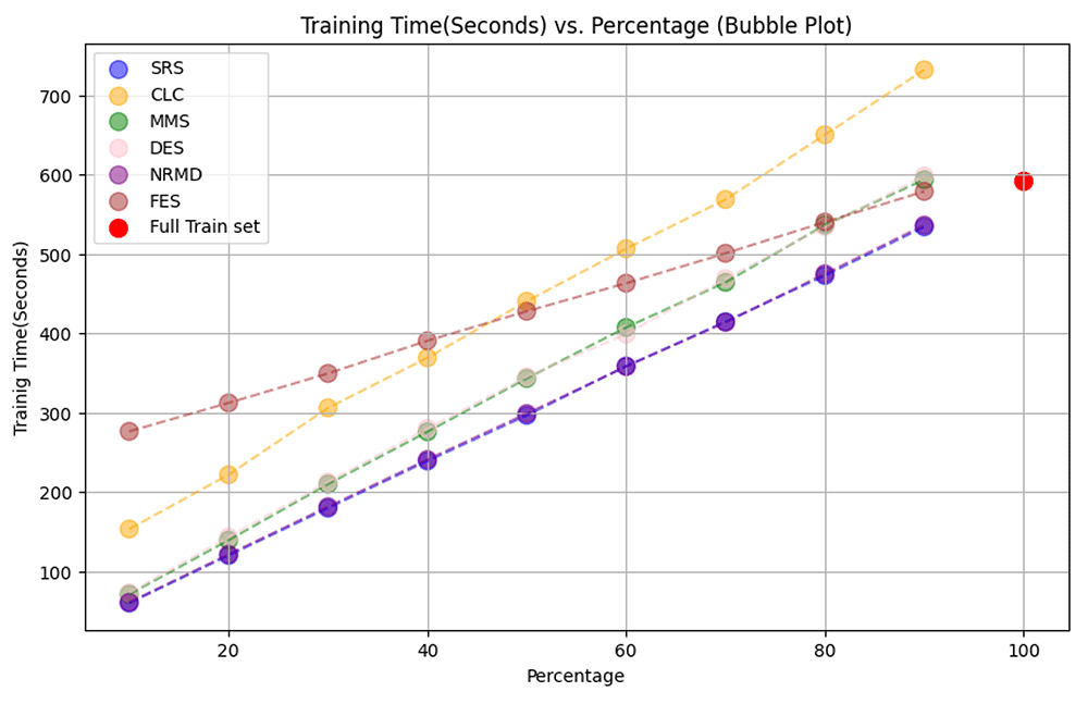
Figure 2. Collision: Reduction + training time.
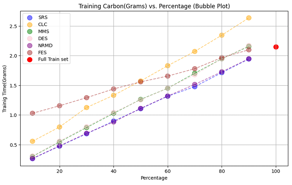
Figure 3. Collision: Reduction + training carbon.
Regarding the ε-representativeness of the reduced datasets with respect to the whole training dataset, the median results can be seen in Figure 4. The first thing we can observe is that MMS reduction is always the best at preserving the ε-representativeness for all the possible reduction ratios, which seems natural if we recall the definition of ε-representativeness and the way the MMS method selects each new example in the reduced dataset. CLC reduction also gives us datasets with good ε values. In contrast, NRMD is the data reduction method with the highest ε values for all the possible reduction ratios.
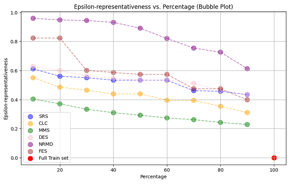
Figure 4. Collision: Reduction + ε-representativeness.
The results on accuracy, macro average precision, macro average recall and macro average F1-score can be seen in Figure 5, Figure 6, Figure 7 and Figure 8 respectively. Regarding accuracy, we can see that the model trained with the whole training dataset has a median success probability of 91%. In general, all the data reduction methods work very well for this dataset. In fact, there are many specific cases where the model obtained with a reduced dataset performs better on the test dataset than the one trained with the full training dataset. We can observe that when the reduction ratio is above 50% the best performing method is FES, while in other cases it is DES. Most of the compared methods manage to maintain accuracy almost intact despite the significant reduction in training size. If we look at the results when we reduce the training dataset to 10% of its size, the model trained after applying DES loses 1.8% of accuracy, while the loss is less than 3% when CLC and SRS are applied. In all cases, this loss in accuracy is more or less linear for all methods except for FES. In this case, the accuracy remains stable while the reduction ratio is high, but it undergoes a drastic drop when a high percentage of examples is removed.
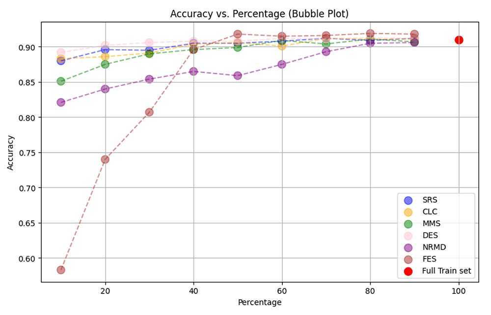
Figure 5. Collision: Reduction + Accuracy.
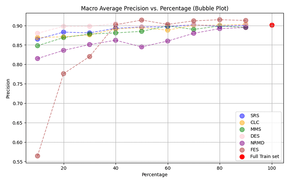
Figure 6. Collision: Reduction + macro average Precision.
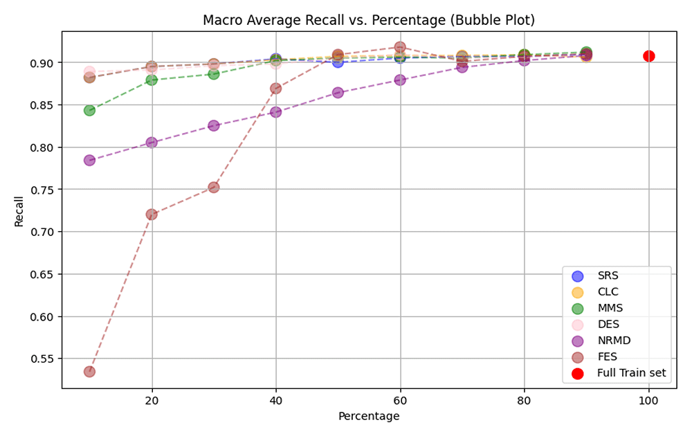
Figure 7. Collision: Reduction + macro average Recall.
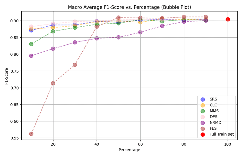
Figure 8. Collision: Reduction + macro average F1-score.
We can observe a similar situation when analyzing the macro average precision. FES is the best method to preserve this metric (even improving the reference case) when the reduction ratio is greater than 50%, while for other ratios the best one is DES. The relationship between macro average precision and training dataset size is also approximately linear for all methods except FES, which suffers a significant drop when the reduction ratio is under 30%.
The results that we get when we analyze the macro average recall are quite different. As we saw with accuracy and macro average precision, this metric is generally well preserved even at very low reduction ratios, although it suffers a very significant drop when FES is applied with a reduction ratio under 30%. But contrary to what we have seen for the previous metrics, no method clearly outperforms the others in terms of macro average recall. All methods except NRMD have given the best median result for some of the chosen reduction ratios.
All the general observations we have made when analyzing accuracy and macro average precision can also be seen for the macro average F1-score. In general, all reduction methods preserve this metric well, being FES the best performing method when the reduction ratio is higher than 50% and DES otherwise. The drop in macro average F1-score is also noticeable when many examples are removed with the FES method, while this tendency is not as pronounced for the other data reduction methods.
Finally, we have found an interesting relationship between the ε-representativeness of the reduced datasets and the macro average F1-score of the models trained with them. Given any reduction ratio p = 0.1, ⋯ , 0.9, we have got the ε-representativeness and the macro average F1-score for each reduction method and each iteration in the experiment (in total there are 6 reduction methods × 10 iterations = 60 pairs (ε,F1) for each p). We computed for each p the Spearman’s rank correlation coefficient64 of its respective cloud of 60 points to test if there exists a dependence between ε-representativeness and the macro average F1-score that can be described with a monotonic (always increasing or always decreasing) function. This coefficient is a real number ρ ∈ [−1, 1], where ρ close to 1 indicates a strong positive monotonic correlation, ρ close to −1 indicates a strong negative monotonic correlation, and ρ close to 0 indicates no monotonic correlation. We also compute the associated p-value to test if the correlation ρ is significantly different from 0. A p-value under a certain threshold (in our case 0.05, which is a standard choice) indicates that ρ is unlikely to be 0, while a p-value above it suggests that the observed correlation might be coincidental and not due to a true dependence between both variables. We performed this statistical analysis independently for each p to eliminate the possible effect that the reduction ratio could have if we used all the possible pairs (ε, F1) altogether.
The results that we got can be seen in Table 3. All the computed ρ values are negative, although they are only significantly different from zero when the reduction ratio is below 40%. That indicates that, when data reduction methods remove a large number of examples, the best performing models are those trained with the reduced datasets that best preserve the ε-representativeness of the entire training set. In a few words, when we reduce the Collision dataset with a small reduction percentage, the smaller the ε value, the better the model will perform.
Table 3. Collision: Correlation between ε-representativeness and macro average F1-score.
This table displays the non-parametric Spearman correlation coefficient and its p-value. Note that when the reduction ratio is equal to or less than 40%, the p-value is below the significance level of 0.05.
| 10% | 20% | 30% | 40% | 50% | 60% | 70% | 80% | 90% |
|---|
| Spearman’s ρ | -0.38 | -0.43 | -0.42 | -0.39 | -0.22 | -0.15 | -0.19 | -0.07 | -0.14 |
| p-value | 0.0 | 0.0 | 0.0 | 0.0 | 0.1 | 0.24 | 0.14 | 0.58 | 0.3 |
Dry Bean Dataset The median results for the computing time and carbon emission can be seen in Figure 9 and Figure 10. There is also a proportional relation between the computation time and the carbon emission in this experiment since each minute of computations emitted approximately 0.21 g of CO2 into the atmosphere. As happened with the Collision dataset, the use of data reduction methods prior to network training helped to reduce the computation time and the carbon emission of the model building with respect to the reference case. The only exception to this rule is when we apply PRD reduction with a reduction ratio greater than 70% (see in Figure 9 and Figure 10). In that situation, both the computation time and the carbon emission of reduction and training exceed those of the reference case. There is no reduction method that runs faster than all the others for this dataset. SRS, MMS, DES, NRMD and CLC run equally fast for the Dry Bean dataset. They hardly need any time to reduce the training data set, so almost all the measured time and, therefore, the carbon emission correspond to the network training.
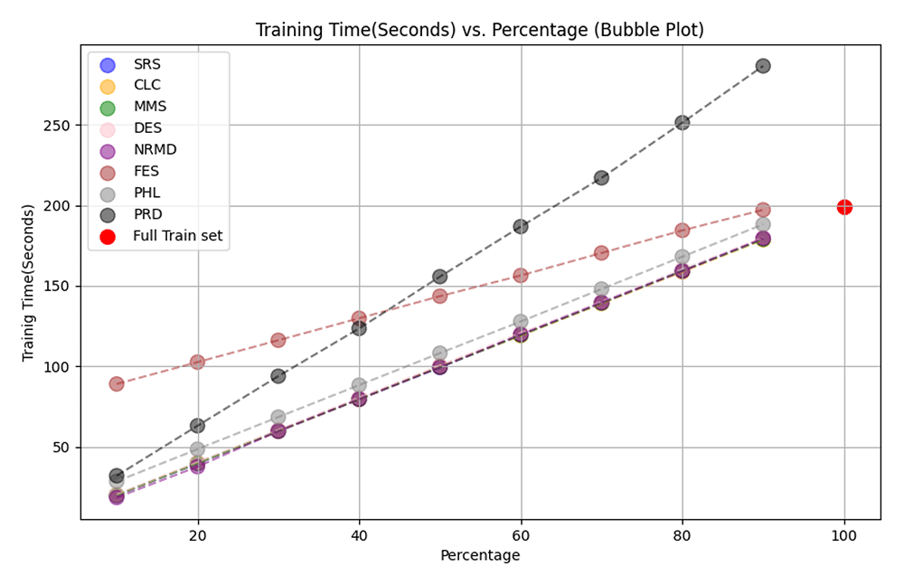
Figure 9. Dry Bean: Reduction + training time.
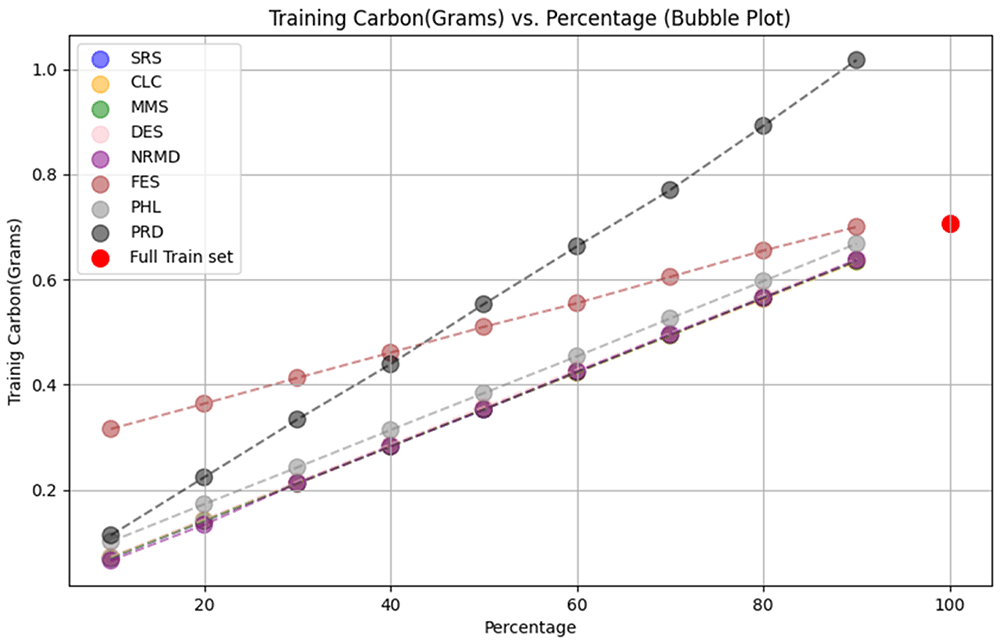
Figure 10. Dry Bean: Reduction + training carbon.
The median values on the ε-representativeness, which can be seen in Figure 11, show us similar results to those observed with the Collision dataset. MMS is still the best data reduction method to preserve the ε-representativeness with respect to the full training dataset, being CLC the second best option. On the contrary, NRMD and PRD are the two methods that generally produce the less ε-representative reduced datasets.
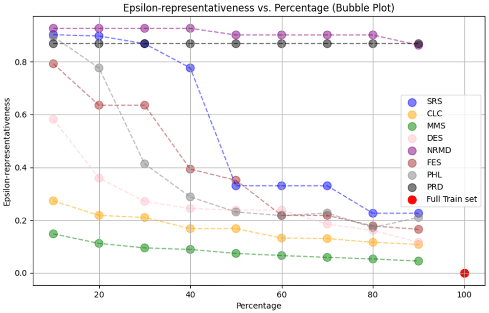
Figure 11. Dry Bean: Reduction + Epsilon.
The median results on accuracy, macro average precision, macro average recall and macro average F1-score for the Dry Bean dataset can be seen in Figure 12, Figure 13, Figure 14 and Figure 15 respectively. In this experiment, the reference case has a median accuracy of 89.9% on the test dataset and, contrary to the Collision dataset, no model trained on a reduced dataset improves this value. No reduction method outperforms the others for every reduction ratio in terms of accuracy. What we observe is that, while, in general, the accuracy is well preserved when the reduction ratio is high, it suffers a drastic drop when many examples are removed from the training dataset. If we wanted to lose at most 5% of accuracy (i.e., have at least 84.9%) we would have to select at least 40% of the data, and not all reduction methods would guarantee this maximum loss of accuracy.
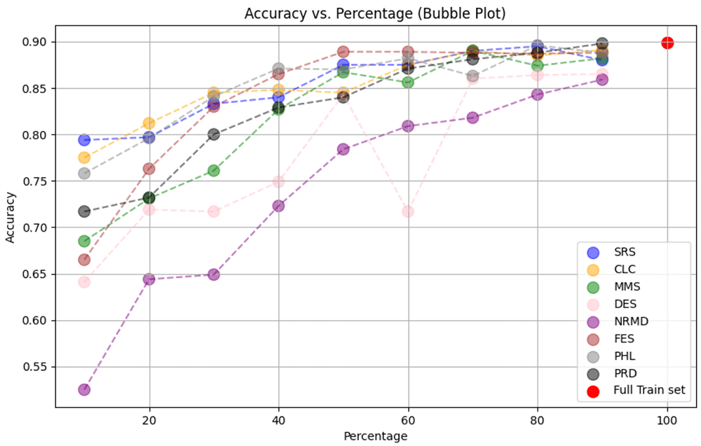
Figure 12. Dry Bean: Reduction + Accuracy.
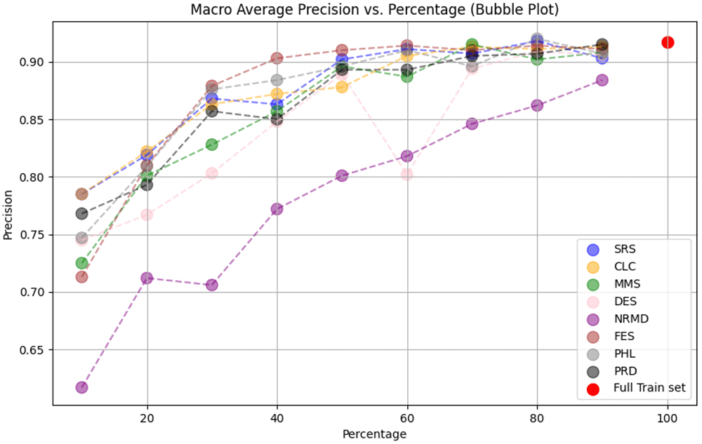
Figure 13. Dry Bean: Reduction + Precision.
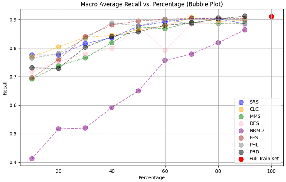
Figure 14. Dry Bean: Reduction + Recall.
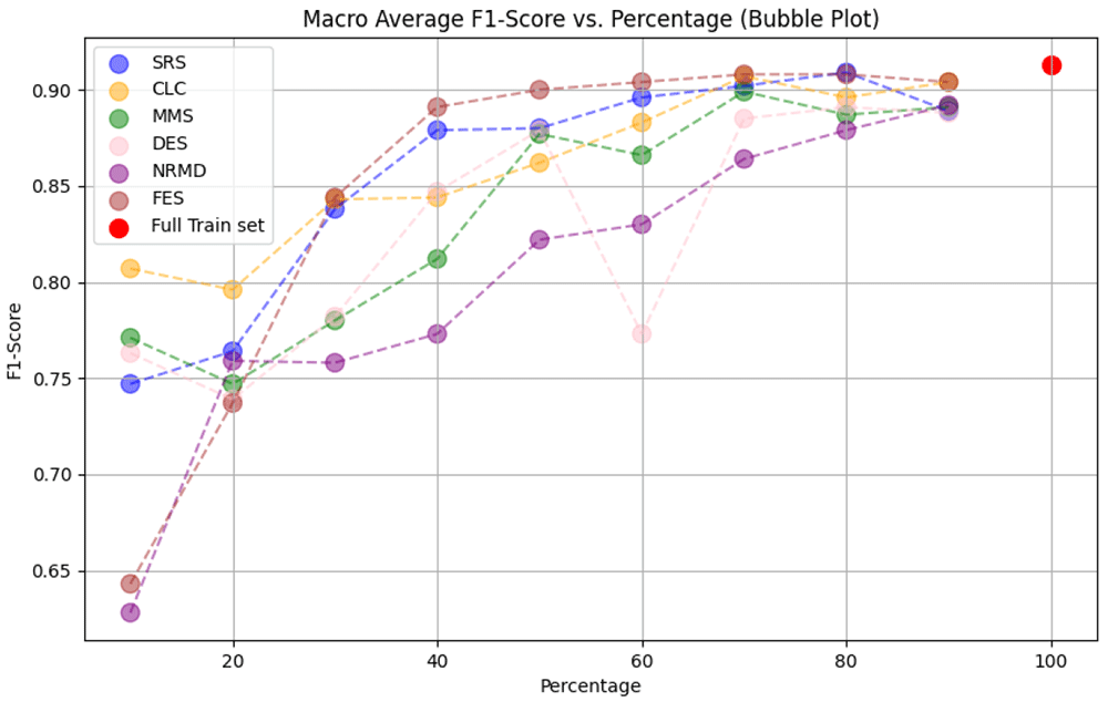
Figure 15. Dry Bean: Reduction + F1-Score.
Regarding the macro average precision, we also find that no method is clearly better than the rest for all reduction ratios, although FES seems to dominate the statistics for the central ratios (30% ≤ p ≤ 60%). Here, the drop in the metric as the reduction ratio decreases is not as pronounced as it is for accuracy. This could be because the macro average precision is a more robust measure as it is less influenced by the larger classes.
We can see similar results when we analyze the details on macro average recall. No method outperforms all the rest, and SRS, PRD, CLC, PHL and FES give the best result for at least one reduction ratio.
Finally, when analyzing the macro average F1-score, we observe that four methods (PRD, CLC, PHL and FES) give the best score for some reduction ratio, but FES seems to give the best performing reduced datasets for 30% ≤ p ≤ 70%. As we said when we analyzed the accuracy, it is not possible to extract a reduced dataset with 30% of its size or less without losing more than 5% of macro average F1-score.
Description of the data structure for accessing the final results The results of both experiments were stored in a Python dictionary with a nested structure, which we will call the results dictionary. On the first level, the result dictionary is composed of 10 dictionaries containing a dictionary for each iteration. The dictionary of each iteration has a dictionary for each data reduction method used. The dictionary of each data reduction method contains an item for each reduction ratio p = 0.1, ⋯ , 1.0, and each one of them is a dictionary containing all the results obtained for that data reduction method and the reduction ratio p in that iteration. The results obtained when the training dataset is not reduced are stored in the item with key p = 1.0. Finally, the dictionary associated with a specific iteration, data reduction method, and reduction ratio, contains a key for the following metrics:
For each class k:
– pre_k: To store the model precision for class k over 𝒟test
– rec_k: To store the model recall for class k over 𝒟test
– f1_k: To store the model F1-score for class k over 𝒟test
pre_avg: To store the model macro average precision for class k over 𝒟test
rec_avg: To store the model macro average recall for class k over 𝒟test
f1_avg: To store the model macro average F1-score for class k over 𝒟test
Once we have this results dictionary, the next step is to summarize the information from all the iterations in a simpler dictionary. This object, which we call the median results dictionary, has the same structure as the entry that we got for each iteration in the results dictionary. For each data reduction method and each reduction ratio, the entry of a specific metric is the median value of the 10 metrics obtained during the 10 different iterations of the experiment. This way we can obtain a more stable representation of the performance of each method across iterations, mitigating the potential influence of outliers or variability in each individual run. All the figures we have seen in this subsection present the metrics from the median results dictionary.
5.2 Experiments for object detection
In this subsection, we describe the methodology we have used in our experiments to extend data reduction techniques to images. Note that we need to adapt the methodology depending on the type of data reduction method. Later, we present the datasets used for the object detection experiments, including the parameter settings and the setup, and finally, we discuss the results that we have obtained.
5.2.1 Methodology
The proposed methodology for the non-wrapper methods, illustrated in Figure 16, consists of the following five steps:
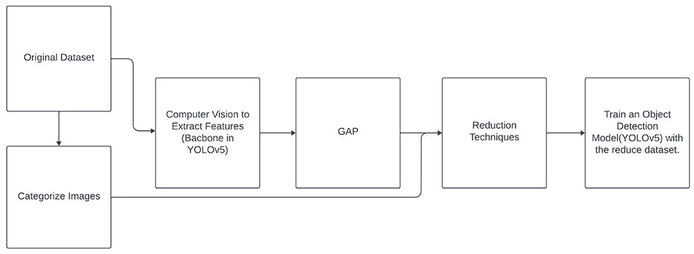
Figure 16. Diagram of the workflow for the proposed methodology to apply data reduction techniques on images dataset.
1. Feature extraction: The objective of this step is to convert the raw pixel values of the images into a set of meaningful and concise features that capture relevant information. These features should allow the model to distinguish between different patterns, objects, or structures within the images. This process involves utilizing a computer vision model, to extract features from all the images in the training set. In our case, we used a pre-trained YOLOv5 model on the COCO dataset (Common Objects in Context)65, a widely used collection in computer vision. The COCO dataset, consisting of approximately 330,000 annotated images with object location and category information, is one of the largest and most diverse datasets available for object detection and segmentation tasks. Utilizing pre-trained models on COCO proves advantageous because of its scale and diversity. This pre-training allows models to learn generic features and representations from a vast array of real-world images, enhancing their ability to generalize across various downstream tasks. This approach can lead to improved performance and efficiency when fine-tuning or adapting these models to specific applications.
2. Categorizing images: In this step, we categorize each image based on the objects present in them. This categorization is essential for applying data reduction techniques, as explained in Section 5.2.2, where we detail how each dataset is categorized.
3. Global Average Pooling: Regarding the output of step 1, we apply global average pooling10,66 to the output of the last layer of the backbone, in order to transform the feature maps into an n-dimensional vector representing their extracted features. Subsequently, these feature vectors can be used to calculate distances or similarities between images, and reduction methods can be applied to them.
4. Applying data reduction technique: Reduction techniques are applied to reduce the amount of samples in the dataset with a specified reduction rate on the matrix produced in step 3, comprising x images and n dimensions, along with the labels from step 2.
5. Fine tuning with the reduced dataset: This step allows us to assess whether satisfactory performance is achieved, potentially maintaining the same level as with the complete training set. The performance evaluation is conducted on the test set using YOLOv5 pre-trained on the COCO dataset, with the backbone frozen. In this context, "fine-tuning with a specific part frozen" implies that some of the model’s parameters are kept fixed during the training process on the new task. This approach leverages prior knowledge gained during initial training, enabling more efficient adaptation to the new task without completely discarding previously learned information.
When using wrapper methods, we must adopt a slightly different methodology than the one previously described (see Figure 17). Initially, we need to categorize the images, similar to the preceding methodology, since these images are intended for object detection and lack specific labels, instead featuring multiple elements within them. Then, we build a straightforward classification model, incorporating the reduction technique during training to yield the reduced dataset. Finally, we train the YOLOv5 detection model using the reduced dataset, aligning with the objective of Step 5 in the aforementioned methodology.
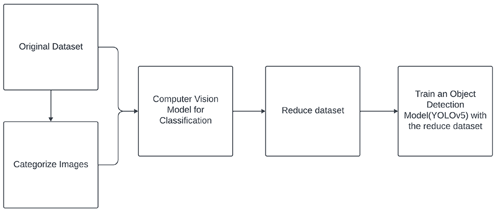
Figure 17. Diagram of the workflow for the proposed methodology to apply wrapper methods.
In addition, to apply the CLC method to images, we introduce a slight modification by applying KMeans67 on X with c (the number of classes) clusters. Then, we determine the number of samples closest (based on the Euclidean distance) to each centroid, resulting in our reduced dataset 𝒟R guided by the specified reduction rate. This adjustment is necessary because the centroids generated by the KMeans method, derived from the representations obtained by our image methodology, do not correspond to specific images from our dataset. Consequently, they do not convey information about what we genuinely aim to detect and localize. This modification is called Representative KMeans (RKM).
5.2.2 Datasets for object detection
Roboflow The Roboflow dataset1 68 comprises 514 RGB images, each 416 pixels in both height and width. These images show pedestrians and people in wheelchairs. The training dataset comprises 463 RGB images, in which a total of 499 pedestrians (annotated as P) and 616 wheelchair users (annotated as W) appear. The test dataset is composed of 51 RGB images, in which a total of 55 pedestrians and 65 wheelchair users appear. The following table shows the criteria that we have used to label the images in the Roboflow dataset according to their content.
| Number of P | Number of W | Label |
|---|
| 0 | 1 | 0 |
| ≥ 1 | 0 | 1 |
| ≥ 1 | ≥ 1 | 2 |
| 0 | ≥ 2 | 3 |
Mobility Aid The Mobility Aid dataset2 69 is composed of 17079 RGB images, of which 10961 are part of the training dataset and the 6118 remaining are part of the test dataset. In this dataset we can find five types of objects: pedestrians (8371, it will be annotated as P), wheelchair users (6458, it will be annotated as W), people pushing a wheelchair (3323, it will be annotated as PW), people with crutches (5374, it will be annotated as C) and people with a walking-frame (7649, it will be annotated as WF). The test dataset is composed of 6208 P, 1993 W, 782 PW, 1883 C, and 2174 WF. The following table shows the criteria that we have used to label the images in the Mobility Aid dataset according to their content.
| Number of P/PW | Number of W/C/WF | Label |
|---|
| 1 | 0 | 1 |
| 0 | 1 | 2 |
| ≥ 1 | 0 | 3 |
| 0 | ≥ 1 | 4 |
| ≥ 1 | ≥ 1 | 5 |
5.2.3 Parameter setting
For the fine-tuning of YOLOv5, we maintain the backbone frozen (pre-trained on the COCO dataset) while training the rest of the model. We configure the training with 100 epochs for the Roboflow dataset and 50 epochs for the Mobility Aid dataset. The batch size is set at 16, and the image size is fixed at 640. We use the SGD optimizer, and the learning rate is set to 0.01 for both datasets. The number of object classes to be detected depends on the specific dataset, being 2 for the Roboflow dataset and 5 for the Mobility Aid dataset.
5.2.4 Experiments setup
We used Python 3.9 and PyTorch27 on Ubuntu 20.04 to perform our experiments. The training phase was executed on an NVIDIA QUADRO RTX 4000 with 8 GB of RAM and an Intel Xeon Silver 4210 preprocessor. Data partitioning followed the default specifications for each dataset.
To assess the performance difference between the full training set and the reduced set, we performed five training runs on the reduced training dataset. We calculated the arithmetic mean and standard deviation of the results for the test set to measure the performance of each reduction method. For the Roboflow dataset, due to its limited sample size, we applied rate reductions of 50% and 75%. In contrast, for the Mobility Aid dataset with a larger sample size, we applied rate reductions of 75% and 90%.
5.2.5 Comparison metrics
We use five metrics to assess the performance of training YOLOv5 with the full dataset compared to training it with different reduction methods and reduction rates. Initially, we use three performance metrics: precision, recall, and mean average precision setting a confidence threshold of 0.5 (mAP@0.5), which means that only detections with a confidence of 50% or higher are considered correct. These metrics are computed individually for each class and globally by averaging the values across all classes. Additionally, we consider the time required for data reduction, measured in seconds for each reduction method, and the model fine-tuning time. Our primary goal with these metrics is to determine whether we can maintain similar performance while considering the time saved.
Furthermore, we calculate ε-representativeness to measure how well the reduced dataset 𝒟R represents the original dataset 𝒟. We also compute carbon emissions during both the data reduction and fine-tuning processes.
5.2.6 Results and discussion
The source code to implement data reduction techniques in these datasets is available at 9 in the ObjectDetection folder.
Roboflow Dataset In our initial experiment, we compared the performance of fine-tuning with the full training dataset against training with a reduced dataset using different reduction methods. Table 4 shows the reduction time, ε-representativeness of the 𝒟r, training time, model performance, and CO2 emissions during the training and reduction phases at a 50% reduction rate. We can observe that, despite training with only 50% of the data, we maintained performance comparable to using the entire dataset. In addition, we reduced the training time by approximately 40%, decreasing from 9 minutes and 20 seconds to about 5 minutes and 45 seconds with 50% of the samples. This reduction in time was accompanied by a similar reduction (about 40%) in CO2 emissions throughout the process. The emission during the application of the reduction methods was small compared to the training time. Notably, effective methods in this scenario include SRS, DES, MMS, RKM, and FES. On the contrary, NRMD and PHL perform worse, with a slight loss of performance. Data reduction times were generally low, except for FES, which showed excessive duration compared to other methods. Conversely, a lower ε-representativeness did not seem to be critical for performance improvement or degradation.
Table 4. Table results for Roboflow dataset and 50% reduction rate.
The ’Precision’, ’Recall’ and ’mAP@.5’ columns show the mean and standard deviation values for the specified variables. The ’CO2(g)’ column indicates the grams of CO2 emitted during the application of the reduction method and during the fine-tuning. The ’R Time(s)’ column shows the time in seconds for data reduction, while the ’FT Time’ column displays the time spent on fine-tuning the model. We have highlighted in red the values obtained during fine-tuning with the full dataset, which serves as a reference. Additionally, we have highlighted in green the best reduction method for each metric.
| Method | R Time(s) | ε | FT Time | Precision | Recall | mAP@.5 | CO2(g) |
|---|
| - | - | - | 9m 19s | A: 0.951±0.001
P: 0.926±0.022
W: 0.976±0.015 | A: 0.897±0.019
P: 0.832±0.031
W: 0.96±0.018 | A: 0.944±0.009
P: 0.906±0.014
W:0.984±0.005 | 5.5 |
| SRS | 0.002 | 2.58 | 5m 44s | A: 0.945±0.021
P: 0.921 ±0.035
W: 0.97±0.011 | A:0.897 ±0.019
P: 0.836±0.03
W: 0.958±0.015 | A:0.897 ±0.019
P: 0.836±0.03
W: 0.958±0.015 | 0+3.3 |
| DES | 0.29 | 3.12 | 5m 44s | A: 0.94±0.001
P: 0.925±0.015
W: 0.95±0.015 | A: 0.885±0.015
P: 0.795±0.03
W: 0.975±0.015 | A: 0.945±0.005
P:0.905±0.005
W: 0.985±0.005 | 0.002+3.3 |
| NRMD | 0.09 | 2.27 | 5m 47s | A: 0.925±0.015
P: 0.905±0.02
W: 0.945±0.02 | A: 0.89±0.016
P: 0.82±0.014
W: 0.956±0.019 | A: 0.932±0.009
P: 0.892±0.016
W: 0.972±0.007 | 0.001+3.3 |
| MMS | 0.09 | 1.99 | 5m 46s | A: 0.951±0.01
P: 0.921±0.017
W: 0.981 ±0.005 | A: 0.894±0.015
P: 0.821±0.029
W: 0.967±0.011) | A: 0.939±0.006
P:0.9±0.011
W: 0.981±0.006 | 0.0004+3.26 |
| RKM | 1.26 | 1.25 | 5m 45s | A: 0.948±0.005
P:0.907±0.015
W: 0.99 ±0.009 | A: 0.895±0.017
P: 0.819±0.032
W: 0.971±0.008 | A: 0.94±0
P: 0.894±0.003
W: 0.985±0.002 | 0.005+3.3 |
| PRD | 0.92 | 1.67 | 5m 44s | A: 0.944±0.02
P: 0.916±0.04
W: 0.97±0.008 | A: 0.89±0.015
P: 0.814±0.025
W: 0.965±0.008 | A: 0.937±0.007
P: 0.894±0.015
W: 0.974±0.008 | 0.002+3.29 |
| PHL | 0.64 | 2.85 | 5m 38s | A: 0.942±0.028
P: 0.9±0.045
W: 0.982±0.014 | A: 0.863±0.21
P: 0.773±0.041
W: 0.954±0.01 | A: 0.927±0.006
P: 0.875±0.017
W: 0.978±0.011 | 0.004+3.24 |
| FES | 8.14 | 2.28 | 5m 39s | A:0.921±0.013
P: 0.871±0.026
W: 0.972±0.017 | A: 0.903±0.011
P: 0.844±0.018
W: 0.962±0.006 | A: 0.948±0.004
P: 0.913±0.009
W: 0.986±0.003 | 0.08+3.24 |
Table 5 shows the same analysis with a 75% reduction rate, where the overall training time was reduced from 9.5 minutes to approximately 4 minutes, a 60% increase in speed. Data reduction time remained insignificant, with some methods displaying longer computation times, such as FES. Despite a slight decrease in performance across all metrics with all methods, SRS, MMS, RKMEANS, and PHL emerged as more robust options. In particular, SRS is the one that best maintains precision and mAP. On the contrary, NRMD showed the most significant loss of performance loss. A lower ε-representativeness did not appear to be a determining factor for better or worse performance. CO2 emissions were also reduced by 60%. On average, the overall mAP for reduction methods showed only a 3% reduction compared to the substantial computational time and CO2 emission savings of 60%. In Figure 18, the mean mAP values for each category and method, along with the full dataset, illustrate the best performing methods. At a 50% reduction rate, performance is nearly maintained, while at a 75% reduction rate, some performance loss is evident. SRS stands out as the most effective method. In addition, a general improvement in accuracy is observed for wheelcharis compared to people, potentially attributed to a slight imbalance in the dataset between the two object categories. We only present the mAP figure (Figure 18) because it is the most comprehensive performance metric for evaluating object detection.
Table 5. Table results for Roboflow dataset and 75% reduction rate.
The Precision’, ’Recall’ and ’mAP@.5’ columns show the mean and standard deviation values for the specified variables. The ’CO2(g)’ column indicates the grams of CO2 emitted during the application of the reduction method and during the fine-tuning. The ’R Time(s)’ column shows the time in seconds for data reduction, while the ’FT Time’ column displays the time spent on fine-tuning the model. We have highlighted in red the values obtained during fine-tuning with the complete dataset, which serves as a reference. Additionally, we have highlighted in green the best reduction method for each metric.
| Method | R Time(s) | ε | FT Time | Precision | Recall | mAP@.5 | CO2(g) |
|---|
| - | - | - | 9m 19s | A: 0.951±0.001
P: 0.926±0.022
W: 0.976±0.015 | A: 0.897±0.019
P: 0.832±0.031
W: 0.96±0.018 | A: 0.944±0.009
P: 0.906±0.014
W :0.984±0.005 | 5.5 |
| SRS | 0.001 | 2.7 | 4m 2s | A: 0.931±0.013
P:0.9±0.017
W: 0.963±0.021 | A: 0.886±0.013
P: 0.815±0.016
W: 0.957±0.01 | A: 0.937±0.005
P: 0.906±0.008
W: 0.968±0.004 | 0+2.25 |
| DES | 0.24 | 3.21 | 3m 59s | A: 0.894±0.022
P: 0.824±0.04
W: 0.964±0.03 | A: 0.86±0.031
P: 0.761±0.045
W: 0.96±0.019 | A: 0.919±0.006
P: 0.855±0.009
W: 0.984±0.005 | 0.002+2.24 |
| NRMD | 0.09 | 2.3 | 3m 58s | A: 0.901±0.016
P: 0.887±0.021
W: 0.914±0.023 | A: 0.846±0.018
P: 0.743±0.043
W: 0.949±0.011 | A: 0.908±0.009
P: 0.857±0.016
W: 0.958±0.003 | 0.001+2.23 |
| MMS | 0.05 | 2.3 | 4m | A: 0.935±0.012
P: 0.927±0.017
W: 0.943±0.015 | A: 0.858±0.009
P: 0.776±0.002
W: 0.94±0.01 | A: 0.922±0.01
P: 0.885±0.019
W: 0.958±0.006 | 0.0004+2.23 |
| RKM | 1.22 | 1.18 | 3m 52s | A: 0.908±0.015
P: 0.821±0.029
W: 0.995±0.006 | A: 0.881±0.009
P: 0.829±0.019
W: 0.934±0.009 | A: 0.927±0.007
P: 0.881±0.015
W: 0.972±0.004 | 0.005+2.18 |
| PRD | 0.38 | 2.68 | 4m | A: 0.895±0.024
P: 0.849±0.038
W: 0.941±0.02 | A: 0.872±0.033
P: 0.793±0.066
W: 0.951±0.011 | A: 0.916±0.013
P: 0.856±0.022
W: 0.967±0.014 | 0.001+2.22 |
| PHL | 0.67 | 3.74 | 3m 59s | A: 0.897±0.02
P: 0.816±0.034
W: 0.977±0.017 | A: 0.887±0.016
P: 0.834±0.023
W: 0.941±0.016 | A: 0.923±0.004
P: 0.877±0.007
W: 0.97±0.004 | 0.004+2.23 |
| FES | 8.63 | 3.12 | 3m 55s | A: 0.884±0.002
P: 0.824±0.033
W: 0.945±0.016 | A: 0.874±0.014
P: 0.796±0.024
W: 0.951±0.009 | A: 0.911±0.008
P: 0.854±0.013
W: 0.968±0.004 | 0.08+2.17 |
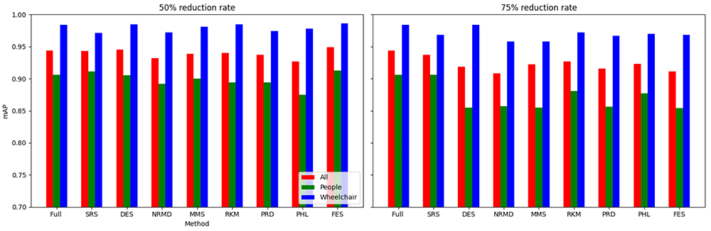
Figure 18. mAP values on Roboflow dataset when using a 50% reduction rate (first column) and when using a 75 percent reduction rate (second column).
Based on the results obtained from this dataset, we can affirm that the application of reduction methods within the proposed methodology, followed by the fine-tuning of YOLOv5 for object detection, led to a significant reduction in CO2 emissions and computation time. Importantly, this reduction did not adversely affect the model’s performance in object detection tasks.
Mobility Aid Dataset Initially, we observe the training benchmark results with the full dataset comprising 10,961 instances. This yields commendable results, such as a mean average precision of 0.93, with a narrow standard deviation of 0.003 across all classes. In particular, the performance stands out in the category of people in wheelchairs (W), surpassing the overall average, while the performance in other categories is noteworthy. Other categories were not included in Table 6 and Table 7 In general, superior performance is evident for the wheelchair, push-wheelchair, and walking-frame categories compared to the pedestrian and crutches categories, which show below-average performance.
Table 6. Table results for Mobility Aid dataset and 75% reduction rate.
The ’Precision’, ’Recall’ and ’mAP@.5’ columns show the mean and standard deviation values for the specified variables. The ’CO2(g)’ column indicates the grams of CO2 emitted during the application of the reduction method and during the fine-tuning. The ’R Time(s)’ column shows the time in seconds for data reduction, while the ’FT Time’ column displays the time spent on fine-tuning the model. We have highlighted in red the values obtained during fine-tuning with the complete dataset, which serves as a reference. Additionally, we have highlighted the best reduction method for each metric.
| Method | R Time(s) | ε | FT Time | Precision | Recall | mAP@.5 | CO2(g) |
|---|
| - | - | - | 2h 8m | A: 0.91±0.008
W: 0.994±0.001 | A: 0.875±0.007
W: 0.896±0.01 | A: 0.93±0.003
W: 0.941±0.003 | 73.85 |
| SRS | 0.006 | 0.86 | 1h 2m | A: 0.912±0.007
W: 0.979±0.029 | A: 0.876±0.007
W: 0.887±0.011 | A: 0.932±0.004
W: 0.94±0.003 | 0+34.12 |
| DES | 7.98 | 0.87 | 1h 2m | A: 0.91±0.009
W: 0.989±0.005 | A: 0.876±0.006
W: 0.893±0.004 | A: 0.93±0.006
W: 0.941±0.001 | 0.04+34.1 |
| NRMD | 3.83 | 1.04 | 1h 2m | A: 0.857±0.004
W: 0.986±0.007 | A: 0.83±0.006
W: 0.865±0.031 | A: 0.903±0.004
W: 0.932±0.002 | 0.015+33.94 |
| MMS | 5.88 | 0.66 | 1h 2m | A: 0.911±0.006
W: 0.994±0.003 | A: 0.875±0.004
W: 0.891±0.007 | A: 0.928±0.005
W: 0.939±0.005 | 0.03+34.13 |
| RKM | 31 | 0.74 | 1h 2m | A: 0.845±0.013
W: 0.961(0.008 | A: 0.795±0.006
W: 0.871±0.008 | A: 0.89±0.006
W: 0.92±0.005 | 0.023+34.1 |
| PRD | 457 | 0.59 | 1h 1m | A: 0.912±0.011
W: 0.989±0.005 | A: 0.876±0.007
W: 0.889±0.008 | A: 0.931±0.004
W: 0.939±0.002 | 1.82+33.91 |
| PHL | 314 | 0.9 | 1h 3m | A: 0.912±0.007
W: 0.994±0.003 | A: 0.875±0.009
W: 0.896±0.003 | A: 0.931±0.003
W: 0.38±0.001 | 1.79+35.09 |
| FES | 289 | 1 | 56m 33s | A: 0.912±0.004
W: 0.993±0.001 | A: 0.875±0.005
W: 0.887±0.009 | A: 0.928±0.004
W: 0.939±0.003 | 2.9+31.83 |
Table 7. Table results for Mobility Aid dataset and 90% reduction rate.
The ’Precision’, ’Recall’ and ’mAP@.5’ columns show the mean and standard deviation values for the specified variables. The ’CO2(g)’ column indicates the grams of CO2 emitted during the application of the reduction method and during the fine-tuning. The ’R Time(s)’ column shows the time in seconds for data reduction, while the ’FT Time’ column displays the time spent on fine-tuning the model. We have highlighted in red the values obtained during fine-tuning with the complete dataset, which serves as a reference. Additionally, we have highlighted the best reduction method for each metric.
| Method | R
Time(s) | ε | FT Time | Precision | Recall | mAP@.5 | CO2(g) |
|---|
| - | - | - | 2h 8m | A: 0.91±0.008
W: 0.994±0.001 | A: 0.875±0.007
W: 0.896±0.01 | A: 0.93±0.003
W: 0.941±0.003 | 73.85 |
| SRS | 0.018 | 1.15 | 48m 31s | A: 0.894±0.01
W: 0.993±0.003 | A: 0.867±0.007
W: 0.886±0.015 | A: 0.926±0.002
W: 0.942±0.002 | 0+26.13 |
| DES | 8.13 | 1 | 43m 28s | A: 0.875±0.014
W: 0.971±0.02 | A: 0.862±0.007
W: 0.893±0.011 | A: 0.917±0.006
W: 0.94±0.003 | 0.04+24.06 |
| NRMD | 2.69 | 1.18 | 43m 17s | A: 0.826±0.005
W: 0.976±0.008 | A: 0.773±0.02
W: 0.846±0.02 | A: 0.873±0.009
W: 0.923±0.005 | 0.017+23.93 |
| MMS | 2.9 | 0.84 | 43m 26s | A: 0.904±0.006
W: 0.996±0.001 | A: 0.875±0.004
W: 0.87±0.01 | A: 0.927±0.004
W: 0.935±0.002 | 0.017+24.06 |
| RKM | 22.92 | 0.95 | 43m 26s | A: 0.812±0.008
W: 0.968±0.007 | A: 0.767±0.012
W: 0.855±0.024 | A: 0.858±0.004
W: 0.918±0.003 | 0.024+24.04 |
| PRD | 66.4 | 1 | 43m 28s | A: 0.908±0.01
W: 0.99±0.006 | A: 0.868±0.007
W: 0.883±0.01 | A: 0.926±0.007
W: 0.938±0.004 | 0.29+24.05 |
| PHL | 317 | 1.04 | 43m 36s | A: 0.898±0.006
W: 0.989±0.005 | A: 0.869±0.005
W: 0.889±0.007 | A: 0.926±0.003
W: 0.937±0.002 | 1.35+24.11 |
| FES | 269 | 1.46 | 43m 29s | A: 0.906±0.007
W: 0.992±0.005 | A: 0.87±0.005
W: 0.875±0.033 | A: 0.927±0.003
W: 0.936±0.002 | 2.69+24.02 |
Moving on to Table 6, which shows the results for a reduction rate of 75%, we observe a significant reduction in training time, approximately 50%. Reduction times are just seconds for most methods, extending to minutes for PRD, PHL and FES. CO2 emissions also witness a substantial decrease, around 55% for all methods, except for PRD, PHL and FES, which emit more CO2 due to a longer computation time during data reduction. Finally, we were able to maintain the performance achieved with the full training set for all data reduction methods. This underscores the practical significance of these methods in reducing computation time and consequently lowering CO2 emissions during model fine-tuning. The exceptions are the RKM and NRMD methods, which show a decrease in performance.
In Table 7, we present similar results, but this time with a reduction rate of 90%. The primary observation is a decrease in performance across various metrics, including precision, recall, and mean average precision. Notably, while there is an overall loss in performance due to reduced metrics in other categories, the decline in the wheelchair category is comparatively less pronounced. Despite this loss in performance, we managed to cut down the training time to 43 minutes, representing about 67% of the training time without dataset reduction. A corresponding decrease in CO2 consumption is observed. Despite the general decline, certain methods, such as SRS, MMS, PRD, PHL and FES, show a relatively robust maintenance of performance.
A visual representation of the mean mAP values for wheelchairs, overall, and for each method alongside the full dataset is shown in Figure 19. This visualization offers a clearer insight into the methods that yield optimal results. With a reduction rate of 75%, we almost maintain performance in all methods, except NRMD and RKM. However, at a rate of reduction 90%, some loss of performance is evident, highlighting the efficacy of methods such as SRS, MMS, PRD, PHL and FES. In particular, the drop in performance for the wheelchair category is less pronounced compared to other categories. We only present the mAP figure (Figure 19), as it serves as the most comprehensive performance metric for evaluating object detection.
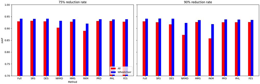
Figure 19. mAP values on Mobility Aid dataset when using a 75% reduction rate(first column) and when using a 90% of reduction rate (second column).
With these results obtained for this dataset, we can confirm that the use of reduction methods within the proposed methodology, followed by fine-tuning YOLOv5 for object detection, led to a significant reduction in both CO2 emissions and computation time. Importantly, this reduction did not affect the model's performance in object detection.