Introduction
Material handling systems using automated guided vehicles (AGVs) are commonly used in manufacturing plants, warehouses, and other facilities (Le-Anh & de Koster, 2006). An important problem in these systems is determining the minimum number of AGVs, or fleet size, necessary to satisfy the effective demand of the logistics process. Several approaches have been proposed to tackle this problem: analytic models (Egbelu, 1987; Fitzgerald, 1985; Groover, 2008), discrete-event simulation studies (Gobal & Kasilingam, 1991; Touran & Taher, 1988; Valmiki et al., 2018), network optimization models (Vis et al., 2001), mixed integer optimization models (Erdogan & Tasan, 2023; Rajotia et al., 1998), heuristic and metaheuristic models (Chawla et al., 2018; Kavakeb et al., 2016; Şenaras et al., 2023; Vivaldini et al., 2016), and regression and other statistical approaches (Arifin & Egbelu, 2000; Beamon & Chen, 1998; Johnson & Brandeau, 1996). Recently, fleet sizing problems have been studied in the context of unmanned aerial vehicles (UAVs), as demonstrated by (Hadas & Figliozzi, 2024).
In this paper we extend the calculus – based or analytic fleet sizing models by treating their parameters as random variables with unknown distributions, characterized only by the first moments (mean and variance). Consequently, the fleet size itself becomes a random variable. By leveraging Taylor series expansions (a well-known technique in statistics, underlying the Delta method (Casella & Berger, 2002)), we derive approximations for both the mean and variance of the fleet size, offering increased accuracy compared to traditional deterministic methods.
This approach bears resemblance to foundational ideas in probability and statistics. For instance, asymptotic expansions such as the Edgeworth and Gram-Charlier series (Johnson et al., 1994; Wallace, 1958) are widely used to refine approximations for random variable distributions using higher-order moments. These techniques provide corrections to the normal distribution, effectively capturing non-normal features like skewness and kurtosis. Similarly, our method systematically expands functions of random variables in terms of their deviations from their means. Taking expectations, the resulting expansions are expressed in terms of the central moments, enabling second-order approximations tailored specifically to the problem of fleet sizing in material handling systems.
We apply our method to the model presented in (Groover, 2008; Körösi et al., 2022), which initially motivated this research. We demonstrate its validity by directly comparing the analytically derived estimates of mean and variance of the fleet size with results obtained from Monte Carlo simulations.
The method has been implemented in the 2nd version of Agent Optimization, a software system developed within the Grow your manufacturing business (Better Factory) Horizon 2020 project. Information about the software implementation can be found in Appendix D.
Static deterministic analytic models for the fleet sizing problem
(Egbelu, 1987) describes four analytic models for the (homogeneous) fleet size estimation problem. The parameters of the models are the number of stations (work centers), the number of loaded trips required between the stations (the flow demand), the distances between stations, the time length of the period or shift, the AGV speed, the time to load and time to unload an AGV, the average efficiency of vehicle after accounting for breakdowns, and in one particular model the blocking time factor and the idle time factor. All models compute a total distance as a sum of the distances between stations weighted by the flow demand between the stations; what mainly distinguishes the models is the way they handle empty-agent trips. Total distance is then divided by the AGV speed and may be adjusted by the efficiency, blocking time, or idle time factors, before adding the loading and unloading times to obtain an ideal cycle time, which is finally divided by the available time (from which perhaps a battery charge time has been subtracted) to yield the desired fleet size.
The model presented in (Groover, 2008) and later in (Körösi et al., 2022), which is what we concentrate in this research on, is quite similar. The model parameters are collected in Table 1:
Table 1. Model parameters used in (Groover, 2008) and in the present study.
| Parameter | Description | Domain |
|---|
| 𝒢(𝒱,ℰ) | A directed graph where 𝒱 = {v1, v2, ... , vn} is the set of vertices, corresponding to
the layout stations, and ℰ ⊂ 𝒱 × 𝒱 is the set of directed edges corresponding to
the direct links between stations, such that (vi, vj) ∉ ℰ for i = j (i.e., no reflexive loops
or self-loops are allowed). | |
| De | The length of the link (direct path) e = (vi, vj) ∈ ℰ, starting at station i and ending at
station j. | De>0 |
| Fe | The average flow rate per hour for the link e = (vi, vj) ∈ ℰ, starting at station i and
ending at station j. | Fe ≥ 0 |
| c | The capacity of an AGV. | c > 0 |
| v | The average speed of an AGV. | v > 0 |
| TL | The average time required to load an AGV. | TL > 0 |
| TU | The average time required to unload an AGV. | TU > 0 |
| A | The AGV availability coefficient. 1 means full availability. | 0 < A ≤ 1 |
| Ft | The traffic factor. 1 means no block due to traffic exists. | 0 < Ft ≤ 1 |
| Ew | The operator efficiency coefficient. 1 stands for the maximum level of efficiency. | 0 < Ew ≤ 1 |
Following (Körösi et al., 2022), we define:
The count of demanded deliveries per hour:
The average distance per loaded trip:
where
The average distance per unloaded trip:
The available time per hour per vehicle:
The total cycle time per delivery per vehicle:
The ideal cycle time per delivery per vehicle:
Then the estimate of the number of vehicles necessary to meet the demand is given by:
This model provides the mathematical background for the Agent Optimization module used in the Horizon 2020 Grow your manufacturing business (Better Factory) project (Körösi et al., 2022).
The impact of variability
An important characteristic of the class of models under discussion is that they treat their parameters as average values, without however mentioning, let alone exploiting, their statistical essence. However, ignoring the fact that the variables in question are random variables is not without risks; for the sake of argument, assume that the distribution of the computed fleet size is close to a normal distribution; then the average value of the fleet size roughly covers the demand of one half of the days. Moreover, as we will soon demonstrate, exploiting the statistical nature of the problem allows for even better estimate of the average necessary fleet size, and provides an approximate quantification of the uncertainty in this estimation.
In all models mentioned above, fij or Fij represents the material transportation demand between stations i and j. Observe that all models contain products of the form fe or Fe, where is a time variable (for example, in all models the loading time TL is multiplied by demand terms), and ratios of the form Σe∈ℰ Fe/v or Σe∈ℰ feDe/v. It is therefore important to study such expressions, focusing on the randomness of the variables involved.
Product of two random variables
From the definition of covariance of two random variables we immediately get the expression for the mean value of their product:
This means that the deterministic approximation using average values is exact only when the variables are uncorrelated.
Ratio of two random variables
The situation is quite different in the case of the ratio of two random variables, because the expected value of the inverse of a random variable X does not equal the inverse of its expected value 1/E[X].
To illustrate this point, we perform a series of tests (simulations), presented in Appendix C.
Discussion
From the above presentation we can conclude that the operations of multiplication and division have distinctly different behavior. The mean value of the product Z = XY of two random variables differs by the product of their mean values only if these variables are correlated. On the contrary, the mean value of the ratio Z = X/Y of two random independent variables X and Y is mainly influenced by the denominator variance, and it can differ significantly from the simple ratio of the mean values of the random variables X and Y.
Very important is also the range of the support of the denominator Y: if the support is not bounded away from 0, the ratio distribution will have some very large values, which will affect both the skewness (asymmetry) and the kurtosis (fat tails or existence of many outliers) of the ratio distribution.
This means that while the variability of quantities such as the total demand will induce a comparable variability to the number of required vehicles N, leaving the mean value unaffected, non-negligent variability and / or skewness of the AGV speed v or some of the efficiency factors A, Ft, Ew can influence both the variance, and the mean value of N.
Analytical estimations based on low-order perturbations
Next, we derive first- and second-order approximations to the mean E[f(X,Y)], and variance Var(f(X,Y)) of a sufficiently differentiable function f(X,Y).
Notation and useful identities. Expansions and the operators 𝒮 and 𝒦
Partial derivatives
As usual, gu will denote the partial derivative of a function g with respect to its argument u: gu ≜ ∂g/∂u.
Deviations from mean, and their products
Let
denote the deviation of a random variable U from its mean.
Some identities related to the expectations of deviations and their products will be used (where we assume that the expectations exist and are finite):
where: μU = E[U], = Var(U), γU and kU are respectively the mean or expected value, the variance, the skewness and the kurtosis of the distribution of U, and σU,V = Cov(U,V) is the covariance of the joint distribution of U and V.
If, in particular, U and V are independent, then for all j = 1,2, ... :
Central moments, mixed central moments, and their order
For all integers i ≥ 2, the i–th central moment of U is the expected value of the i-th power of ϵU:
where pU(u) is the probability density function (p.d.f.) of the distribution of U.
The exponent i is called the order of the moment.
Likewise, for all integers i, j ≥ 1, the (i, j)–th mixed central moment is the expected value of :
where pU,V(u,v) is the joint probability density function of the joint distribution of U and V.
The sum i + j is called the (total) order of the mixed moment.
Order of approximation, approximation of expectations, and remainder. The operators 𝒮 and 𝒦.
Suppose we want to approximate a function f(U,V) by a polynomial ϕ(x, y, z) of degree i in some variables x, y, z, and denote this by the notation ≃i. Using the Bachmann–Landau asymptotic notation:
The variables, with respect to which this approximation is performed, will generally be clear from the context, but they will occasionally be mentioned in the text for clarity. The integer i is the order of approximation.
A common choice of variables is (x, y) = (ϵU, ϵV), in which case ϕ(x, y) is the truncated Taylor series of f(U,V) of order i around (μU, μV), and the expected value of the right-hand side of (19) becomes:
Therefore, a suitable set of variables for approximating expectations is the set of moments of the distributions pU and pV of a specific order, and the mixed moments of their joint distribution pU,V of the same (total) order.
The term in (20) will be called the remainder of the expansion. It consists of terms that are of order i + 1 in the standard deviations and mixed moments:
We will denote by 𝒮i(f) or 𝒮if the i-th order expansion of a function f in terms of the standard deviations and mixed moments of its arguments:
for specific values of the coefficients αm,n and βm,n, with
That is, 𝒮if(U,V) is the sum of a multivariate polynomial of degree i in the standard deviations σU, σV, and a linear combination of the mixed moments of total order up to i.
When the more formal notation 𝒮i is not necessary, we may use the simpler (but not so powerful) notation ≃i, introduced earlier.
It is easy to verify that 𝒮i is linear. Consider any two functions f1, f2 of the random variables U and V expanded according to (23), which we may rewrite as:
Let:
Then, with κ, λ ∈ ℝ:
Therefore,
We will also make use of the operator 𝒦i:
Importantly, the operator Si is idempotent:
For a very simple proof of this (rather obvious) statement: by definition of the 𝒮i operator and the remainder ℛi + 1, for all i ≥ 0:
Applying the linear operator 𝒮i to both sides of (26) yields:
By extension, the operator 𝒦i is also linear.
Mean value approximations
The Taylor expansion of f(X,Y) around the point θ = (μX, μY) is:
Applying the linear expectation operator yields:
where the remainder ℛ3 consists of terms that are of third order in the standard deviations and mixed moments:
From (29), it is straightforward to get the approximations of the mean:
1st order approximation:
2nd order approximation:
Variance approximations
Since
the Taylor expansion of g(X,Y) = f(X,Y)2 is also needed. By the chain rule:
and
Then,
Taking expectations:
By (32), to approximate Var(f(X,Y)) up to 2nd order, we must find a 2nd order approximation of E[f(X,Y)]2:
Therefore,
Hence, we obtain a 2nd order approximation for Var(f(X,Y)):
Higher-order approximations
The second-order approximations ignore the effect of higher-order moments (such as skewness and kurtosis) and mixed moments. Evaluating this effect in the general case requires approximating E[f(X,Y)2] by a fourth-degree polynomial which involves, apart from the moments of X and Y, the mixed moments of their joint distribution up to (total) order 4. In a practical setting, this may be too much to ask for.
Instead, we will compute higher-order approximations of the mean and the variance of the function f(X,Y) for a few important – especially for the problem we are studying – cases.
Sum of correlated variables: f(X,Y) = X + Y
For the sake of completeness, we begin by stating the well – known results:
Product of correlated variables: f(X,Y) = XY
Equation (12) gives the exact formula for the mean value of a product, and is repeated here for convenience:
The variance is given by (32):
The Taylor series expansion of f(X,Y) = XY around (μX, μY) is:
from which the Taylor series of f2 is obtained:
Therefore, and considering (11 – 16):
Hence, the difference between the exact (4th order) variance of the product and its 2nd order approximation
equals , which, in the case of independence, simplifies to :
Inverse of a random variable: f(X,Y) = 1/Y
The Taylor series of 1/Y around Y = μY ≠ 0 is given by:
from which, and if the distribution Y is bounded away from 0, the mean value approximation of fourth order is:
Hence,
For the variance approximation we expand 1/Y2:
so that
Then,
so that
Ratio of independent random variables: f(X,Y) = X/Y
From the previous results and the independence of X and Y it is straightforward to obtain the higher order approximations of the mean value:
The calculation of variance is performed in a similar manner:
The expansions of the second and third term have already been computed (44,45). The first term requires some attention:
Therefore:
Summary of the basic approximations
Table 2 summarizes our results.
Table 2. Mean value and variance approximations for X + Y, X⋅Y, 1/Y and X/Y.
| Z = X + Y | Z = X⋅Y | Z = 1/Y | Z = X/Y
X,Y independent |
|---|
| Mean value | | | | |
|---|
| 1st order | μX + μY
Exact | μX μY
Exact when independent | | |
| 2nd order | | 1st order + σX,Y
Exact | 1st order + | 1st order + |
| 3rd order | | | 2nd order – | 2nd order – |
| 4th order | | | 3rd order + | 3rd order + |
| Variance | | | | |
|---|
| 2nd order |
Exact | | | |
| 3rd order | | 2nd order +
| 2nd order –
| 2nd order –
|
| 4th order | | 3rd order +
Exact | 3rd order +
| 3rd order +
|
| Comments | | When independent, the 4th
order expansion becomes
| Assumes finite
skewness and
kurtosis of the
denominator Y | Assumes finite skewness
and kurtosis of the
denominator Y |
Estimation of the fleet size statistics
We are now ready to apply our analysis to the fleet size problem. In what follows we work with the model (1 – 7) from (Groover, 2008); the method can also in principle be applied to the models (see Appendix B) from (Egbelu, 1987), although such an attempt is not presented in this work.
We begin by modeling the demand variability: for simplicity, we assume that all individual link demands Fe are perfectly correlated and all have the same relative standard deviation δ, so that they all fluctuate by the same percentage around their nominal value. We model this condition by:
where Δ is a random variable having mean value 0 and standard deviation δ, so that indeed
For e, e′ ∈ ℰ, e ≠ e′:
so that the correlation between Fe and Fe′ is indeed
Under this assumption, and treating distances De as constants:
and
Let us compute the mean and variance of these variables:
and
Then,
Hence Ld is constant, as is Le.
Next, we turn our attention to the ideal cycle time per delivery per vehicle:
We obtain in succession:
Since (Ld + Le)/v is independent of TL + TU, from (6) we obtain:
Next, since Tic = wTc, and w, Tc are independent, and using the operators 𝒦0, 𝒦2:
Notice that we retained only the 0th order terms from the approximation of μTC, since the term is the variance of the quantity w, thus already a 2nd order term, and keeping the full 2nd order approximation 𝒮2μTC would contain higher order terms.
By (67), (63) and (65),
and so (since 𝒮2σTc = 𝒦2σTc):
Consider now the available time per hour per vehicle:
Since all variables are independent, the approximations of Tav are easily obtained:
The last equality in (71) means that the 0th-order approximation of μTav is exact.
With 𝒮2μTic, 𝒮2, 𝒮2μTav, 𝒮2 given by (69) – (72), we can approximate the statistics of the fleet size N (given by (8)), taking into account that the variables defining the numerator are independent from those defining the denominator:
The expressions in (73), (74) are approximations based on the 2nd order approximations of the various quantities used. However, they are not 2nd order approximations themselves. The actual 2nd order approximations of μN and σN are (see Appendix A):
where the operator 𝒦0 returns the 0th order terms of its operand (see definition (26)).
From (69):
Keeping only the 0th order terms:
Examples
We apply our results in the examples presented in (Körösi et al., 2022) and (Groover, 2008).
Assume that the AGVs transport raw parts from station 1 to production stations 2, 3, and 4. Some parts must be transported from station 3 to station 4. All production stations send finished parts to unload station 5.
Table 3 contains the data for examples 1, 2, and 3.
Table 3. Data for examples 1, 2, and 3.
| Flow rates (mean values, trips per hour) | 12 = 9, 13 = 5, 14 = 6,
25 = 9, 34 = 2, 35 = 3, 45 = 8 |
| Distances (m) | D12 = 50, D13 = 120, D14 = 205,
D25 = 80, D34 = 85, D35 = 170, D45 = 85 |
| Average distance per unloaded trip (m) | Le = 795 (example 1) OR Le = 100 (examples 2 and 3) |
| Flow rate relative deviation | δ = 25% |
| AGV capacity | c = 1 |
| AGV speed (m/min) | μv = 84
σv = 16.8 |
| Loading time (min) | μTL = 0.5
σTL = 0.12 |
| Unloading time (min) | μTU = 0.5
σTU = 0.12 |
| Loading – unloading time correlation | ρTL,TU = 0.3 |
| AGV availability | μA = 0.95
σA = 0 (examples 1 and 2) OR σA = 0.1 (example 3) |
| Traffic factor | μFt = 0.85
σFt = 0.09 |
| Operator efficiency | μEw = 0.95
σEw = 0 (examples 1 and 2) OR σEw = 0.1 (example 3) |
Initially, we compute:
Assume that each loaded trip from station (i) to station (j) is followed by a trip back to station (i) where the AGV travels unloaded. Then Le = ΣDe = 795. In this setup Le ≫ Ld, which is very inefficient.
Total cycle time per delivery per vehicle Tc = TL + TU + Ld/v + Le/v:
Ideal cycle time per delivery per vehicle Tic = wTc:
The available time per hour per vehicle:
Finally, the fleet size estimates:
For comparison, the deterministic model gives
Example 2: Continuation from example 1, low Le
Assume now that the process is designed to achieve a low (relative to Ld) Le, approximately equal to the length of the link from station 5 to station 1. This requires a two-position platform at each production station, so that a vehicle can pick up a load of finished parts right after each delivery of raw parts.
Therefore, assume that Le = D51 = 100. Repeating the calculation we find:
Total cycle time per delivery per vehicle Tc:
Ideal cycle time per delivery per vehicle Tic = wTc and resulting fleet size:
Example 3: Continuation from example 2, increased denominator variance
Suppose that both AGV availability and operator efficiency have a medium standard deviation: σA = σEw = 0.1. This affects the available time per hour per vehicle, since its variance increases:
The fleet size estimates are now calculated to be:
Resulting fleet size:
Observe that the mean value estimate has increased slightly by 2% because of the increased denominator variance alone, accompanied by an 11% increase in the standard deviation estimate. The denominator standard deviation has increased approximately by 70%.
Table 4 contains the data for example 4.
Table 4. Data for example 4.
| Flow rates (mean values, trips per hour) | 12 = 10, 23 = 15, 31 = 0 |
| Distances (m) | D12 = 50, D23 = 60, D31 = 50 |
| Average distance per unloaded trip (m) | Le = 50 |
| Flow rate relative deviation | δ = 25% |
| AGV capacity | c = 1 OR c = 2 |
| AGV speed (m/min) | μv = 50
σv = 5 |
| Loading time (min) | μTL = 0.75
σTL = 0.08 |
| Unloading time (min) | μTL = 0.5
σTL = 0.05 |
| Loading – unloading time correlation | ρTL,TU = 0 |
| AGV availability | μA = 0.95
σA = 0.09 |
| Traffic factor | μFt = 0.9
σFt = 0.09 |
| Operator efficiency | μEw = 1.0
σEw = 0 |
(i) AGV capacity c = 1:
Total cycle time per delivery per vehicle Tc = TL + TU + Ld/v + Le/v:
Ideal cycle time per delivery per vehicle Tic = wTc, available time per hour per vehicle, fleet size:
(ii) AGV capacity c = 2:
Changing the capacity affects , which in turn affects Tc = (TL + TU) + , Tic = wTc, and N = :
Table 5 contains the data for example 5.
Table 5. Data for example 5.
| Flow rates (mean values, trips per hour) | 12 = 23 = 67 = 200
34 = 36 = 45 = 56 = 100
71 = 0 |
| Distances (m) | D12 = 65, D23 = 45, D34 = 50, D36 = 140
D45 = 70, D56 = 120, D67 = 65,
D71 = 45, |
| Average distance per unloaded trip (m) | Le = 45 |
| Flow rate relative deviation | δ = 25% |
| AGV capacity | c = 1 OR c = 100 |
| AGV speed (m/min) | μv = 50
σv = 5 |
| Loading time (min) | μTL = 0.75
σTL = 0.08 |
| Unloading time (min) | μTL = 0.5
σTL = 0.05 |
| Loading – unloading time correlation | ρTL,TU = 0 |
| AGV availability | μA = 0.95
σA = 0.09 |
| Traffic factor | μFt = 0.9
σFt = 0.09 |
| Operator efficiency | μEw = 1.0
σEw = 0 |
(i) AGV capacity c = 1:
Total cycle time per delivery per vehicle Tc = TL + TU + Ld/v + Le/v:
Ideal cycle time per delivery per vehicle Tic = wTc, available time per hour per vehicle, fleet size:
(ii) AGV capacity c = 100:
Comparison with simulation experiments
We complete this study by comparing the estimates presented in the previous section with results of simulation experiments.
Experiment setup:
We model the distributions of the problem data by symmetric triangular distributions with the specified mean value and variance, except for cases where it is not possible to honor the domain of the respective variable. Such are the cases of A, Ft, and Ew coefficients, the domain of which is bounded below 1, and constructing a symmetric triangular distribution with the specified mean and variance while its support is a subrange of [0,1] may be impossible. In such cases, we model the random variable by a beta distribution, which can meet any requirements of this kind, with the important drawback that its support is not bounded away from zero, so that division by such variables may result in fleet size distribution with large and / or unstable higher order moments.
Δ is modeled as a random variable following a symmetric triangular distribution with support . Indeed, .
Following the Choleski decomposition method (Glasserman, 2003), TL and TU are modeled as:
TL = , where follows a symmetric triangular distribution with the given mean μTL and variance ,
, where follows a symmetric triangular distribution with the given mean μTU and variance . and are independent.
It is easy to show that with this definition, TL and TU have the prescribed means and variances, as well as the prescribed correlation between them:
Obviously, E[TL] = E[] and
Regarding TU:
and, since and are independent:
Then, the correlation between TL and TU is verified:
so that
Having constructed same-size samples of Δ, TL, TU, AGV speed v, AGV availability A, traffic factor Ft, and operator efficiency Ew, the rest of the calculations are straightforward to perform for all sample points.
This way we derive a sample of the distribution of the fleet size N.
The empirical distribution of the ideal cycle time per delivery per vehicle Tic is plotted with a blue solid line, while the one of the available time per hour per vehicle Tav is plotted with a green solid line. Notice that these quantities are the numerator and denominator of the Equation (8), which determines the fleet size.
The empirical distribution of the latter is plotted with a red solid line.
Two ranges are also depicted as shaded areas: the one in blue represents the range within ± 1 standard deviation around the empirical mean, derived from the sample data; the one in red represents approximately the ± 1 estimated standard deviation range around the estimated mean, computed as 2nd order approximations. Although the two ranges do not coincide, they overlap significantly.
Finally, the three vertical straight lines (not always distinguishable from one anther) mark: the empirical mean (a dashed blue line), the 2nd order estimation of the mean (a solid green line), and the 0th order estimation of the mean (a dotted black line).
Example 1 (Table 6, Figure 1):
Table 6. Specifications, sample statistics, and theoretical predictions for example 1.
| Input statistics vs specifications: | Derived samples statistics vs estimations: |
|---|
| |
|
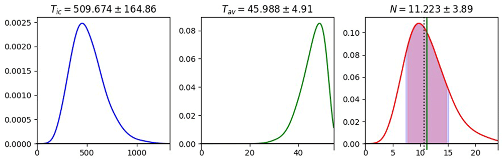
Figure 1. Empirical (sample) distribution of the ideal cycle time per delivery per vehicle (left), the available time (middle), and the fleet size (right) for example 1.
Example 2 (Table 7, Figure 2):
Table 7. Specifications, sample statistics, and theoretical predictions for example 2.
| Input statistics vs specifications: | Derived samples statistics vs estimations: |
|---|
| |
|
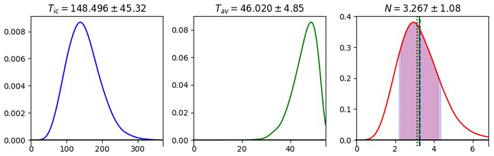
Figure 2. Empirical (sample) distribution of the ideal cycle time per delivery per vehicle (left), the available time (middle), and the fleet size (right) for example 2.
Example 3 (Table 8, Figure 3):
Table 8. Specifications, sample statistics, and theoretical predictions for example 3.
| Input statistics vs specifications: | Derived samples statistics vs estimations: |
|---|
|
|
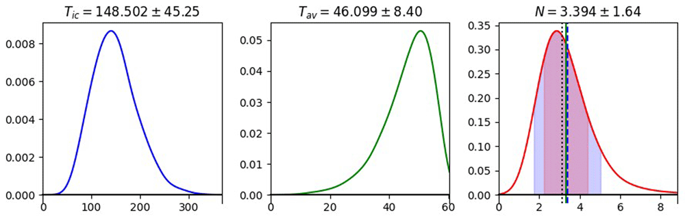
Figure 3. Empirical (sample) distribution of the ideal cycle time per delivery per vehicle (left), the available time (middle), and the fleet size (right) for example 3.
Example 4:
i) AGV capacity = 1 (Table 9, Figure 4)
Table 9. Specifications, sample statistics, and theoretical predictions for example 4i.
| Input statistics vs specifications: | Derived samples statistics vs estimations: |
|---|
| |
|
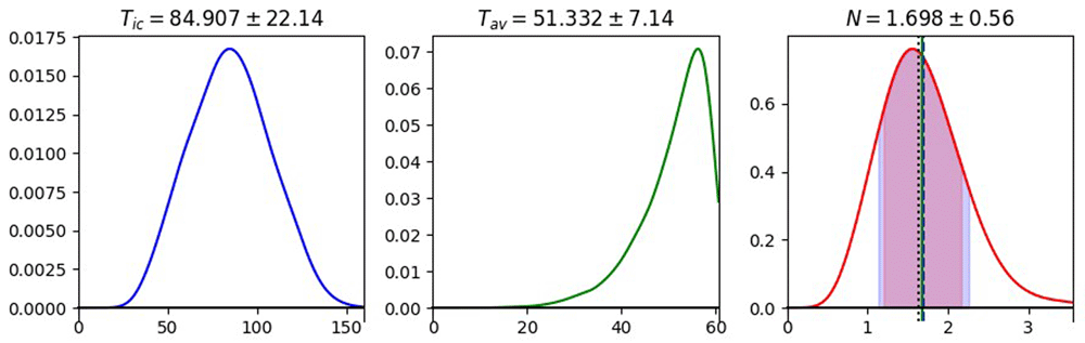
Figure 4. Empirical (sample) distribution of the ideal cycle time per delivery per vehicle (left), the available time (middle), and the fleet size (right) for example 4i.
ii) AGV capacity = 2 (Table 10, Figure 5)
Table 10. Specifications, sample statistics, and theoretical predictions for example 4ii.
| Input statistics vs specifications: | Derived samples statistics vs estimations: |
|---|
| |
|
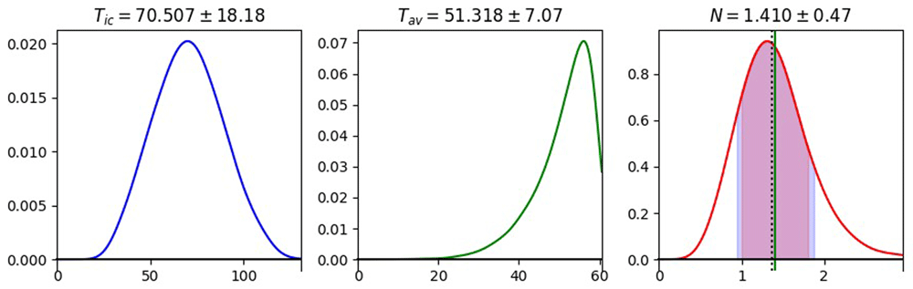
Figure 5. Empirical (sample) distribution of the ideal cycle time per delivery per vehicle (left), the available time (middle), and the fleet size (right) for example 4ii.
Example 5:
i) AGV capacity = 1 (Table 11, Figure 6)
Table 11. Specifications, sample statistics, and theoretical predictions for example 5i.
| Input statistics vs specifications: | Derived samples statistics vs estimations: |
|---|
| |
|
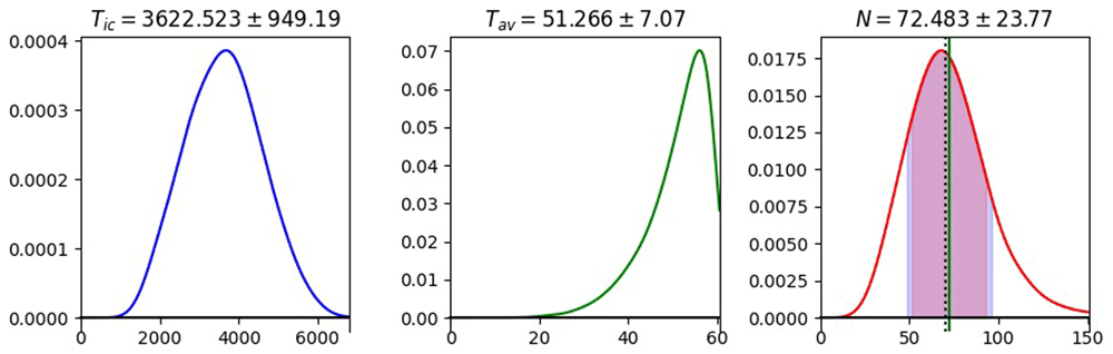
Figure 6. Empirical (sample) distribution of the ideal cycle time per delivery per vehicle (left), the available time (middle), and the fleet size (right) for example 5i.
ii) AGV capacity = 100 (Table 12, Figure 7)
Table 12. Specifications, sample statistics, and theoretical predictions for example 5ii.
| Input statistics vs specifications: | Derived samples statistics vs estimations: |
|---|
| |
|
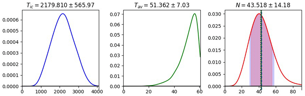
Figure 7. Empirical (sample) distribution of the ideal cycle time per delivery per vehicle (left), the available time (middle), and the fleet size (right) for example 5ii.
Discussion
The simulation experiments verify the validity of the approach. The 2nd order mean value estimation of the fleet size is remarkably accurate. For example, in the last experiment the 0th order (deterministic) estimation is 42.195, the 2nd order estimation is 43.177, while the actual (sample) estimation is 43.518. So, while the deterministic estimation is off by 3%, the 2nd order estimation is less than 1% off. In the third experiment, where the skewness and kurtosis of the N sample are large and perhaps unstable (γN = 7.27, kN = 154.83), the 2nd order mean value estimation is off by only a little more than 2%, a clear improvement over the deterministic estimation which is off by 8%.
The approximation to the fleet size variance is cruder. For example, in the last experiment the variance is estimated to be 12.312, while the sample has variance equal to 14.182, so that the estimation error to the standard deviation is 13.2%. In the more pathogenic third experiment, σN(sample) = 1.64, while the 2nd order variance estimation is 1.102 (a 33% error for the standard deviation estimation). However, even with this relatively high error in the estimation, this is valuable information, since it provides the analyst a systematic way to assess, to a first approximation, the process reliability. Estimating that the fleet size has a high variance might indicate the need for additional AGVs to ensure a higher level of confidence in meeting the effective demand.
Conclusion
This paper presents an extension to traditional fleet sizing models by modeling key inputs as random variables, improving the model's applicability under uncertainty.
Using the expansion of a function of random variables in terms of the central moments of its arguments, we derive second-order approximations of the expected value and the variance of the required number of automated guided vehicles (AGVs). The method yields more accurate fleet size estimates than the deterministic approach, and also enables better-informed decision making and higher confidence in satisfying demand under uncertain conditions.
Several numerical examples, conducted as Monte Carlo simulations, are used to demonstrate the applicability of the method and illustrate various aspects of the problem. The effects of skewness, kurtosis, and support range of the ratio distribution’s denominator are highlighted, and it is pointed out that the mean value is approximated quite satisfactorily, even in cases with high denominator variance, while the variance estimation is accurate only in cases with low denominator variance.
Appendix A – 2nd order approximation of fleet size statistics
Obtaining the 2nd order approximations of μN and σN requires some attention, because the expressions in (73), (74), which use 2nd order approximations of various quantities, when expanded as polynomials in the various random variable moments contain higher order terms as well. To see this, consider first (73):
The first term 𝒮2μTic/μTav is indeed of 2nd order, but the second term is of 4th order.
From (25):
Observe that for all quantities studied in this work, 𝒦1 ≡ 0. On the other hand, 𝒦0 = 𝒮0, so that 𝒦2 = 𝒮2 – 𝒮0. Additionally, for the variance of all quantities U it holds that .
The expression for μN can be written as
Consider now (74), which is trickier:
The first term is already a 2nd order approximation (see also the derivation of (70)). The term ((𝒮2μTic)2/) . is of 6th order, it contains, however, 2nd order terms, which we must keep:
Thus, the 2nd order approximation of is given by
Both expressions differ from (73 – 74) only in that the 2nd order term 𝒮2μTic has been replaced by its 0th order approximation 𝒦0μTic (remember that 𝒦0 = 0, so that 𝒮2 = 𝒦2).
Appendix B – Parameters of the models of (Egbelu, 1987)
For the sake of completeness, the expressions giving the estimate of the required number of vehicles for the four models described in (Egbelu, 1987) are also listed below, somewhat simplified. Besides those used by the previously described model, the variables given in Table B1 are also used:
Table B1. Additional model parameters used in (Egbelu, 1987).
| Parameter | Description | Domain |
|---|
| fij | Expected number of loaded trips required between work center i and work center j
during a shift period. This differs somewhat from Fij of (Groover, 2008), which is flow
rate per hour. | |
| tb | The battery charge time of an AGV. | tb ≥ 0 |
| b | The blocking time factor | 0 ≤ b < 1 |
| γ | The idle time factor. Not to be confused with the skewness of a random variable,
introduced in (14). | 0 ≤ γ ≤ 1 |
| ρ | Vehicle efficiency, after accounting for breakdowns | 0 < ρ ≤ 1 |
| d(αi,βi) | The distance between the delivery station αi and the pickup station βi within the i-th
work center. | d(αi,βi) ≥ 0 |
Appendix C – The effect of denominator variability
In the class of problems we study, among all possible arithmetic operations that are involved in the computation of the required fleet size, the division operation has the most significant effect on both the expected value and the variance of the latter, as it cannot be represented exactly by any finite-order expansion Si(X/Y) of the form (22).
To illustrate this point, we perform a series of tests (simulations). The random variable X is taken to follow a triangular distribution, while the random variable Y is taken to follow either a triangular or a beta distribution, to help illustrate the importance of the support range. We experiment both with the spread of the distributions (the variance), and with their level of asymmetry (skewness).
For each test we define the distributions for X and Y through their parameters: the support endpoints a, b and the mode c for triangular distributions; the shape parameters α and β in the case of the two-parameter beta distributions, the support of which is (0,1).
Then,
The latter values are the estimations of the mean value and the variance of the distribution of Z = X/Y.
For each test, we also provide the low – order approximations of the mean value and the variance of the ratio, computed according to the rules summarized in Table 2.
The results are summarized in Table C1:
We may conjecture that with low denominator variance, the low order approximations of the mean value and variance are quite satisfactory, irrespectively of any skewness of the distributions X and Y. For larger values of the denominator variance, the variance estimation (hence, the estimation of the standard deviation) loses accuracy significantly, and the larger the variance and / or the support of the denominator, the larger the effect on the skewness and kurtosis of the ratio distribution and the error on the variance estimate. Still, the accuracy of the 2nd order estimate of μX/Y is consistently significantly better than the deterministic estimate, 𝒮0μX/Y = μX/μY.
Appendix D – The Agent Optimization application
The method presented in this paper forms the basis for the second version of the Agent Optimization application, developed during our participation in the Horizon 2020 Grow Your Manufacturing Business (Better Factory) project. The original version of the application, presented in (Körösi et al., 2022), implemented the (Groover, 2008) model, as described by Equations (1 – 8). It is a command – line interface application, which reads data from a MongoDB database and calculates the “optimal number of agents”, and is part of the Logistics Library, formerly known as Open Platform for Innovation in Logistics (OPIL).
The new version of the Agent Optimization application, developed by the authors, comes in two variants which can run as Docker containers: a command – line interface (CLI), like the first version, and a Web-based interface (Figure D.1). Both variants use the graph model when editing the quantities Fe and De of the links e = vi, vj (Table 1), provide advanced data validation, allow reading and writing JSON files with the system data directly from / to disk, and encapsulate the underlying database, which becomes an optional component. In a nutshell, the second version facilitates the data manipulation significantly.
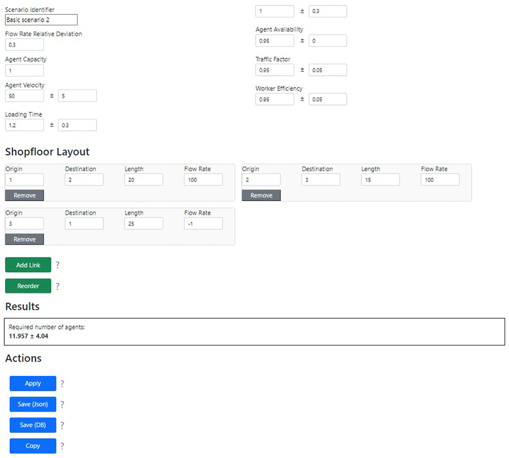
Figure D.1. Partial view of the Web-based user interface.
Figure D.2 depicts a high-level architecture of the system. The Uncertain Quantity Calculator subsystem maintains the mathematical model: mean values, standard deviations, finite or infinite ranges, and random variables encompassing a range (their support), a mean value and a standard deviation. The subsystem knows how to perform certain operations on the random variables: addition, subtraction, multiplication, and division. These are implemented according to the rules summarized in Table 1. Both mean values and variances are approximated up to 2nd order, and the standard deviation is approximated by the square root of the (approximate) variance.
The Agent Optimization Theory subsystem maintains the model (1 – 8) and provides also any covariances required to compute the additions, multiplications, and divisions necessary, making use of the services of the Uncertain Quantity Calculator to perform the actual calculations.
This design allows easy adaptation to other problems that can be solved by a sequence of simple arithmetic operations.
The Agent Optimization application (ver. 2) can be downloaded from the RAMP marketplace (RAMP, n.d.).
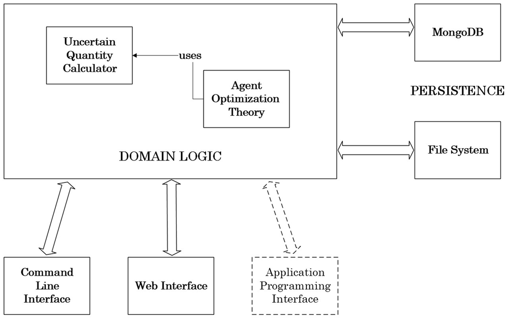
Figure D.2. Agent Optimization (v.2) high-level architecture.